This tutorial aims to give you a definite guide on how to insert checkboxes in Google Sheets.
We will go over the basics, as well as some more advanced topics like conditional formatting with checkboxes, assigning custom values, and counting all the values from checkboxes.
We will even sum everything we know into a real-live example: a simple habit tracker.
Excited? So Am I!
PS. The tutorial should take you around 12-20 minutes to complete. You may follow along using the spreadsheet available here (just make a copy and you are ready to go).
- How to Insert Checkbox In Google Sheets
- Checkbox Data Validation in Google Sheets
- How To Do Conditional Formatting in Google Sheets
- How to Count All Checkboxes in Google Sheets
- How to Make a CheckBox In Google Sheets Mobile App? (iPhone, Ipad, Android)
- Final Task: Create a Habit Tracker
- Some Questions You May Have
- My final thoughts
How to Insert Checkbox In Google Sheets
Inserting a checkbox is actually super simple to do. These are the steps to follow:
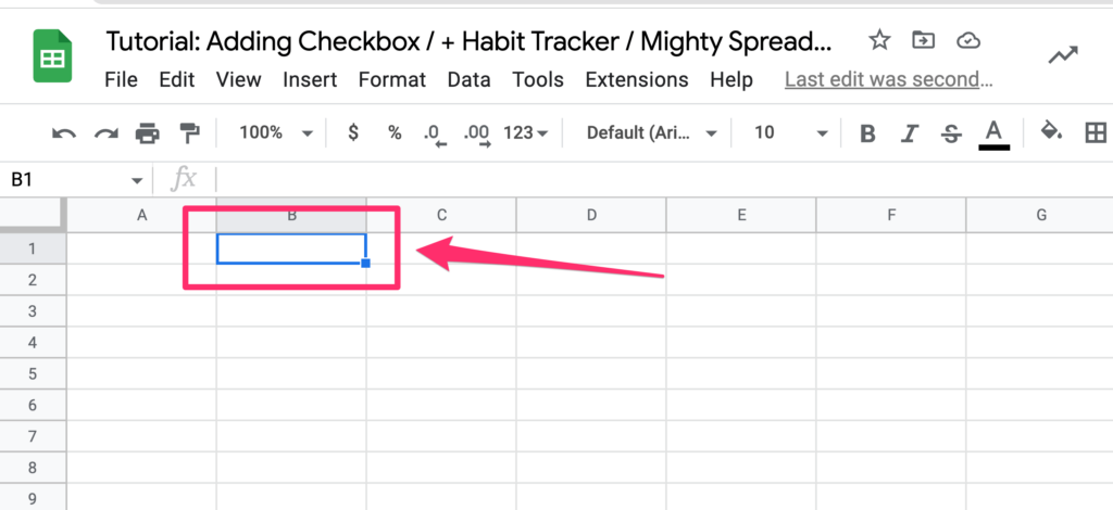
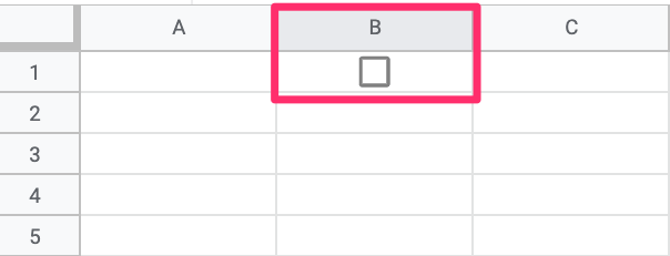
Step 1: Select the cell where you would like it to appear
Step 2: From the Options Menu select Insert and find the checkbox option
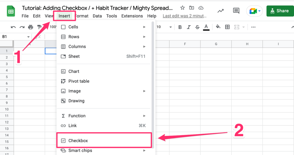
Pro tip: To insert checkboxes in multiple cells simultaneously, select the desired range of cells and then click on Insert in the Options Menu
Checkbox Data Validation in Google Sheets
In this section, we will focus on how to take the value from our checkbox and put it to good use.
Google Sheets Checkbox Default Values (True/False)
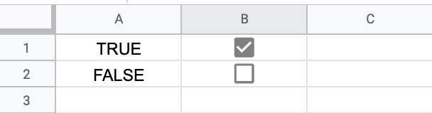
The default values for every checkbox are:
TRUE– when it is checkedFALSE– when it is unchecked
Although it seems super basic it opens a lot of opportunities for you mainly because you can now use the cell value in many different functions such as the IF function or even a SPARKLINE function if you want to be fancy and create a little graph for your data.
Let’s see it in action:
Step 1: Create a checkbox in the B1 cell.
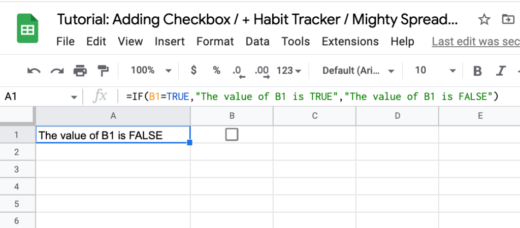
Step 2: In the A1 cell add an IF function to show different values depending on the checkbox status.
This is the IF function that we will use:
=IF(B1=TRUE,"The value of B1 is TRUE","The value of B1 is FALSE")
And this is how it should look like:
Using the IF function is the easiest way to programmatically check if the checkbox is checked or not
Now, let’s move on to customizing the checkbox so you’re not limited to just TRUE and FALSE values.
How To Add Custom Values to Checkbox
In many cases, you may want your checkbox to return a custom value that you will later use in your calculations or conditional statements. Here’s how to do it:
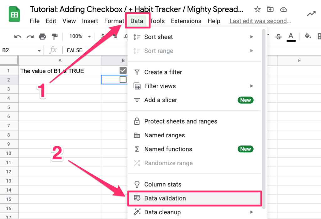
Step 1: Click on the checkbox you’ve created previously or create a new one and focus on it

Step 2: Go to Data > Data validation
Step 3: Make sure that “Criteria” is set to “Checkbox”
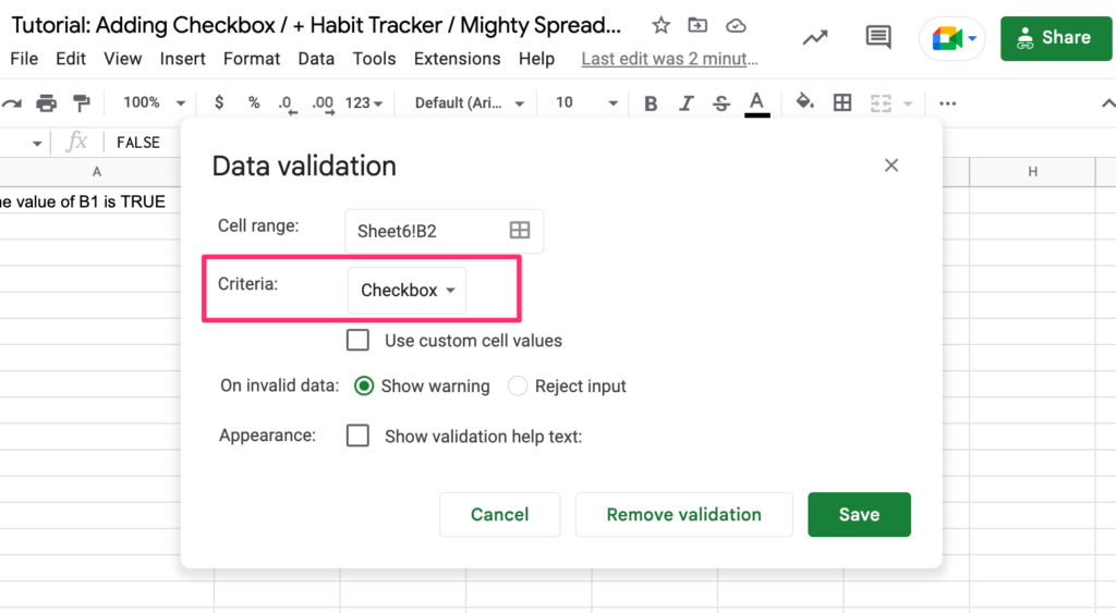
Step 4: Select the “Use custom cell values” checkbox
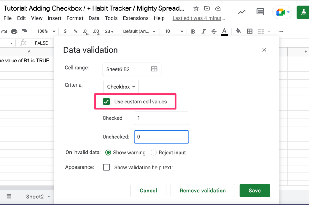
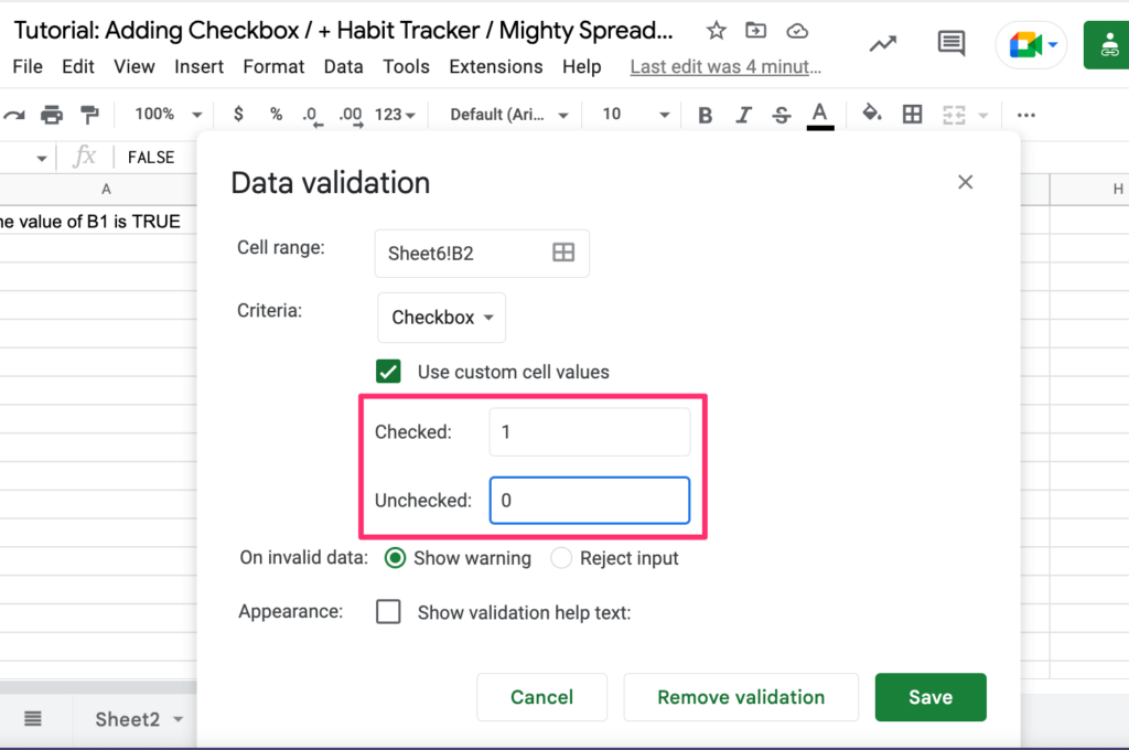
Step 5: Provide custom values for “Checked” and “Unchecked” inputs (in our case they will respectively be 1 and 0) and click on the SAVE button
Now you can use your checkbox exactly the same way but the output will cover the values you provided.
How To Do Conditional Formatting in Google Sheets
Alright, now that you know how to add a checkbox to Google sheets, how to read its value, and use it inside an IF statement let’s focus on putting this knowledge to something more practical.
In this section, we will cover conditional formatting. We will learn how to format one field based on the checkbox value of another field.
Here are some real-life examples that you may find useful:
- Creating a simple to-do app
- Highlighting values
Creating a Simple To-Do App in Google Sheets Using Checkboxes
If you were ever wondering how to highlight a row if the checkbox is checked this is the answer you were looking for:
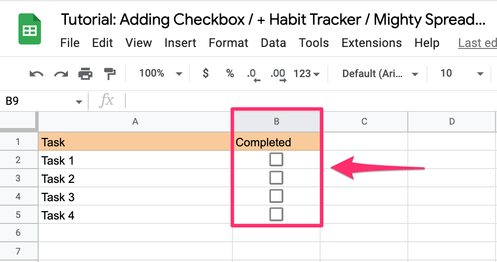
Step 1: Create a list of To-Do tasks in column A
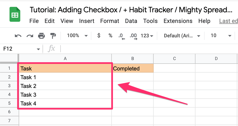
Step 2: Create a set of checkboxes in Column B
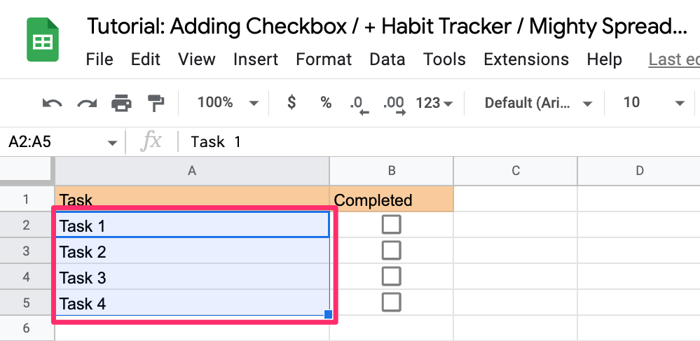
Step 3: Select all tasks from the column A
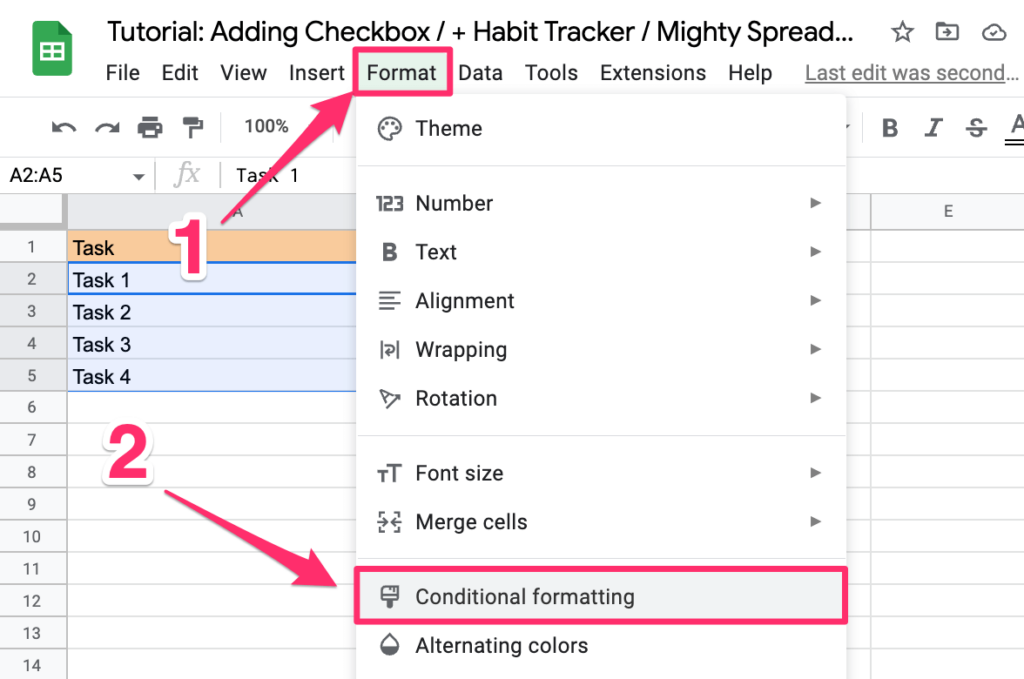
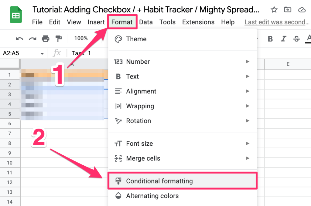
Step 4: Select Format > Conditional formatting from the Options Menu
Step 5: In the popup that will appear on the right side find the “Format Rules” section and in the “Format cells if” section select the “Custom formula is” from the dropdown menu
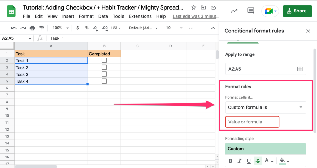
Step 6: In the custom formula input type =B2=TRUE
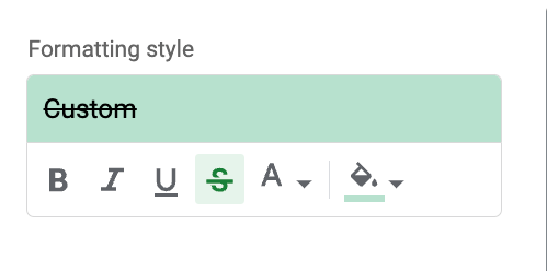
Step 7: Pick your formatting style for completed tasks and click on Done
That’s all you had to do, your small To-Do App is ready to be used 🙂
Highlighting multiple values based on single checkbox status
You can also use conditional formatting in Google Sheets to highlight and analyze your data. It will be quite similar to what we did a second ago but the filter will be toggled by only one checkbox.
Here’s what you need to do:
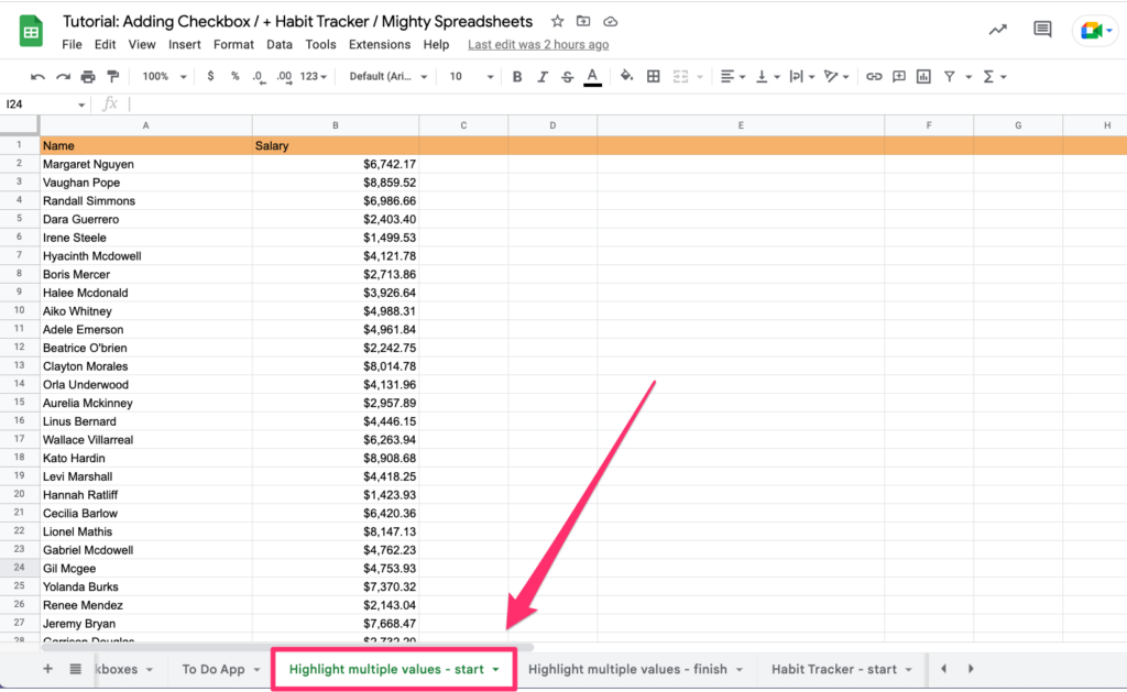
Step 1: Open the “Highlight multiple values – start” worksheet (If you haven’t created a copy of the exercise spreadsheet yet, you can do so here.)
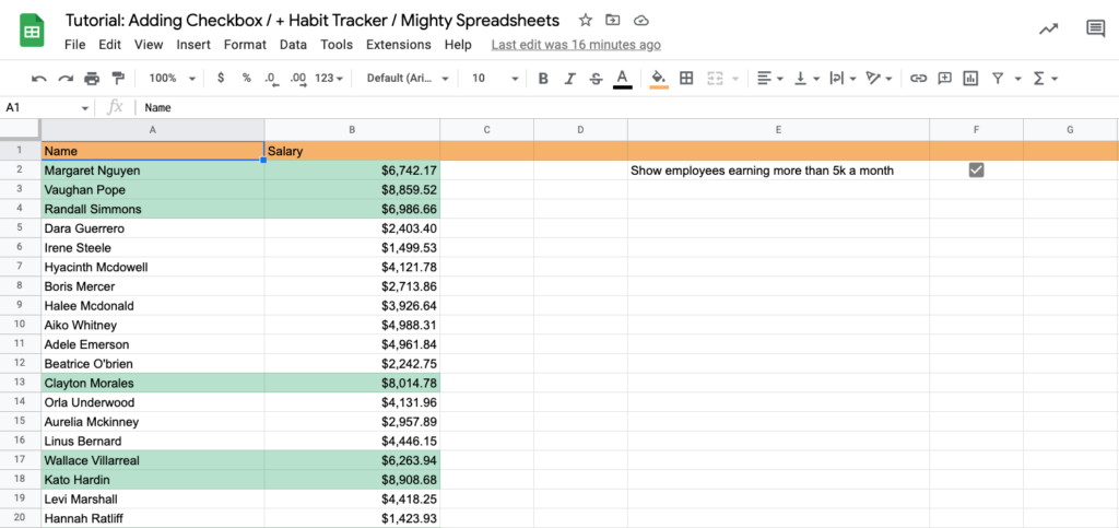
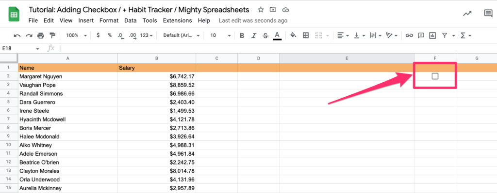
Step 2: Create a checkbox in the F2 cell
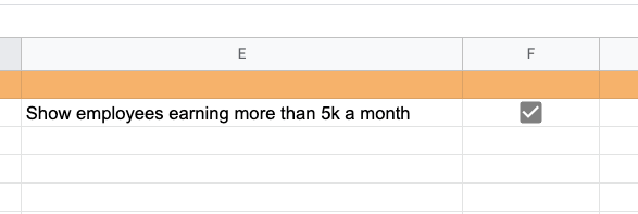
Step 3: Add a description in an E2 cell. In the exercise, I added “Show employees earning more than 5k a month”
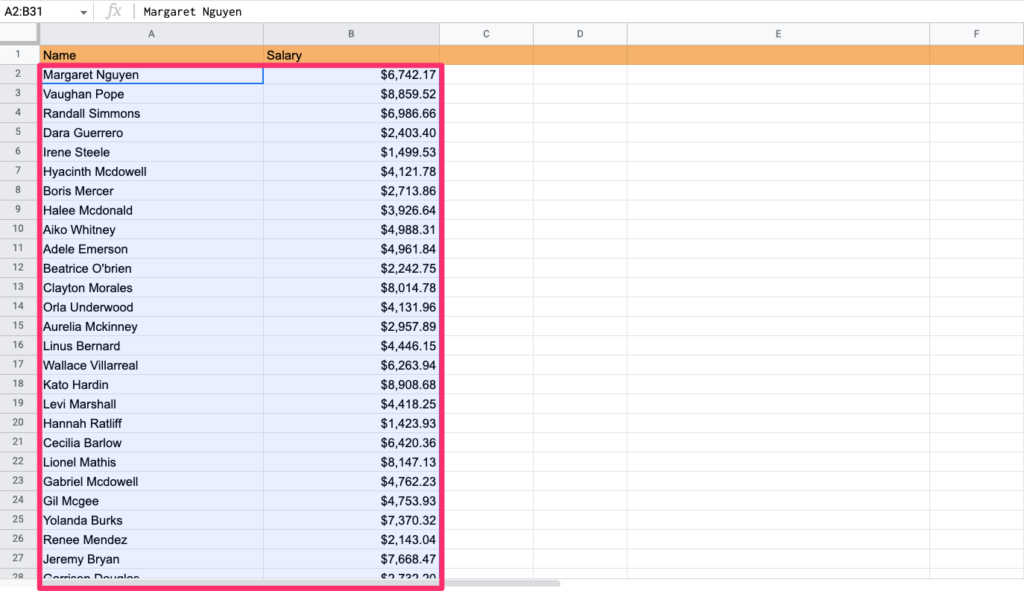
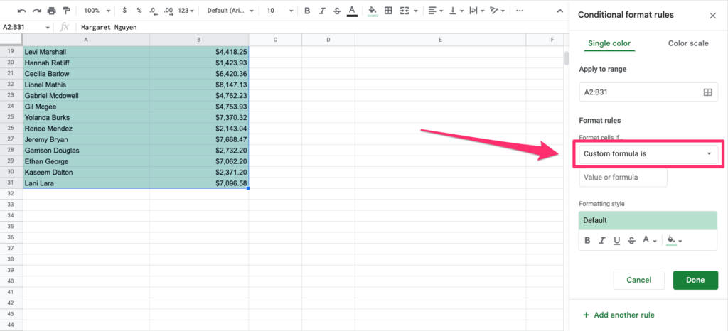
Step 4: Select all the cells you want to apply the logic for. In this exercise, it will be A2:B31
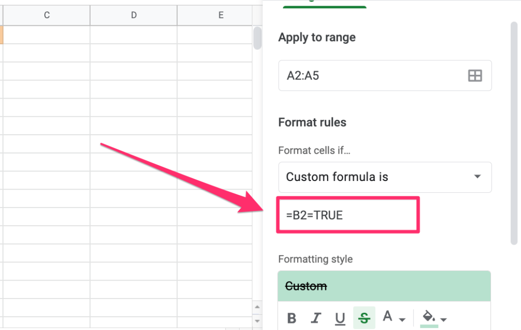
Step 5: Go to Format > Conditional formatting in the Options Menu
Step 6: In the format rules section set the “Format cells if” to “Custom formula is”
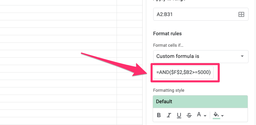
Step 7*: Add the formula: =AND($F$2,$B2>=5000) and click “Done”
Step 8: Use your checkbox to see if the values are highlighted
*I probably owe you a bit of explanation on what we did in step 8:
- AND formula returns
TRUEonly when all provided criteria areTRUE(andFALSEwhen at least one of them doesn’t match) - The
$sign before the column name and row number ($F$2) tells Google Sheets to use that specific cell value for all cells in our data set. - The
$sign in the second argument ($B2>5000) ensures the checkbox is referenced correctly and that the checks are only applied to the values in Column B
This is our final output:
How to Count All Checkboxes in Google Sheets
COUNTIF is a quick and easy way to count all selected checkboxes in your sheets.
It returns the number of cells in a range that meet certain criteria.
And here’s the syntax for this function: COUNTIF(range, criterion)
Where:
range– is your selection of fieldscriterion– is your pattern that you want to check the fields against
Let me break it down by giving you an example:
Step 1: Open the “Count all checkboxes – start” worksheet
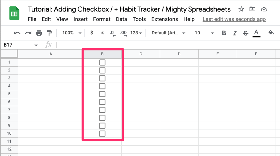
Step 2: Create a set of 10 checkboxes in Column B
Step 3: Apply =COUNTIF(B1:B10, TRUE) function to the B12 cell
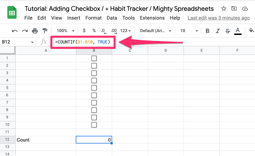
The function sums up all cells with a value of TRUE in a range between B1 and B10.
How to Make a CheckBox In Google Sheets Mobile App? (iPhone, Ipad, Android)
Unfortunately, you can’t create a checkbox on your iPad or iPhone using the Google Sheets App for Apple devices because it doesn’t support data validation at the moment of writing this article. Hopefully, data validation for IOS will be supported in the future.
However, you can easily add checkboxes if you are an Android phone owner. To do so, just follow these steps:
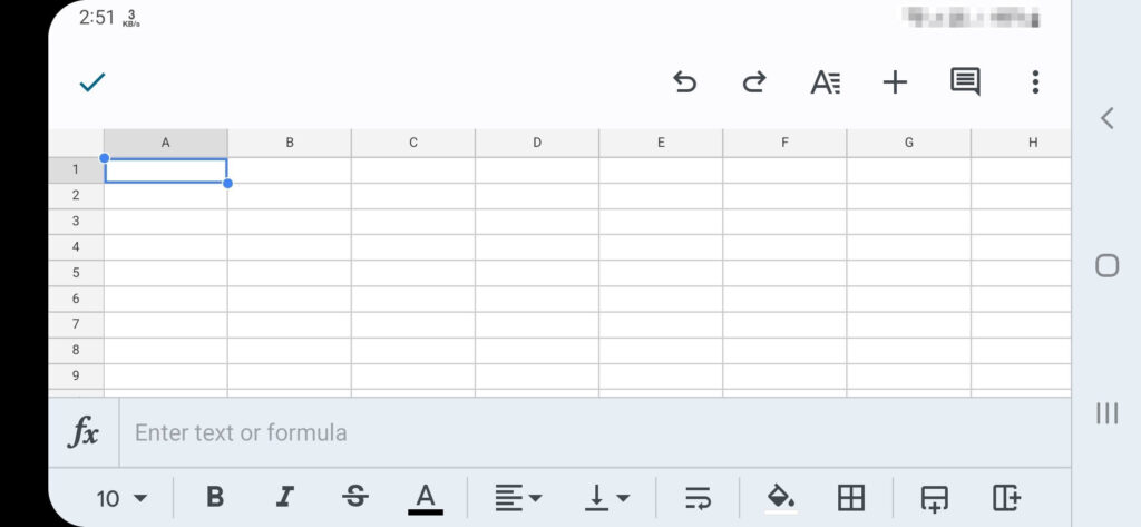
Step 1: Select the cell where you want to add your checkbox
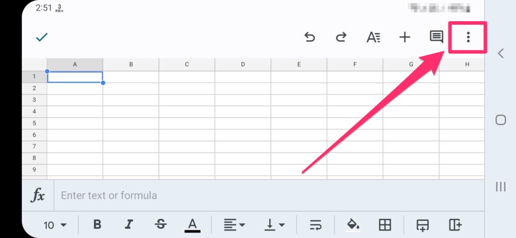
Step 2: Click on the three dots in the upper-right corner of your screen
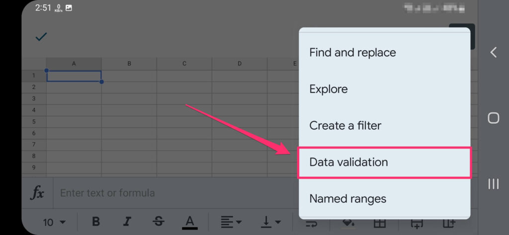
Step 3: From the menu that will appear select “Data validation”
Step 4: Change the criteria to “Checkbox” and click on “Add/Save” (at the top)
Final Task: Create a Habit Tracker
In our final task, we will create a simple habit tracker app.
Here are the features that we are going to cover:
- We will determine the number of tasks completed each day.
- We will calculate the number of tasks we were unable to complete each day.
- We will calculate the % value of tasks completed each day so that you can identify the most productive days for you.
Let’s start!
Step 1: Open the “Habit Tracker – start” worksheet
Step 2: Add checkboxes for all tasks and every day of the week (B3:H9 range)
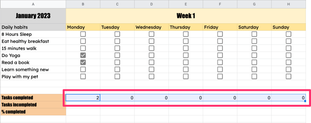
Step 3: Focus on the B12 cell and add a formula that will count all checkboxes with TRUE as their value (we covered this in the previous section).
Step 4: Spread the formula to other cells in this row (just drag and pull the small blue rectangle that is visible in the bottom right corner of the selected B12 cell)
Step 5: Now let’s do a similar operation in the B13 cell, just count all checkboxes with the value of FALSE
Step 6: In a similar way spread the formula across the row
Step 7: Let’s calculate the % value.
Focus on the B14 cell and add this formula: =COUNTIF(B3:B9,TRUE)/COUNTA(B3:B9)
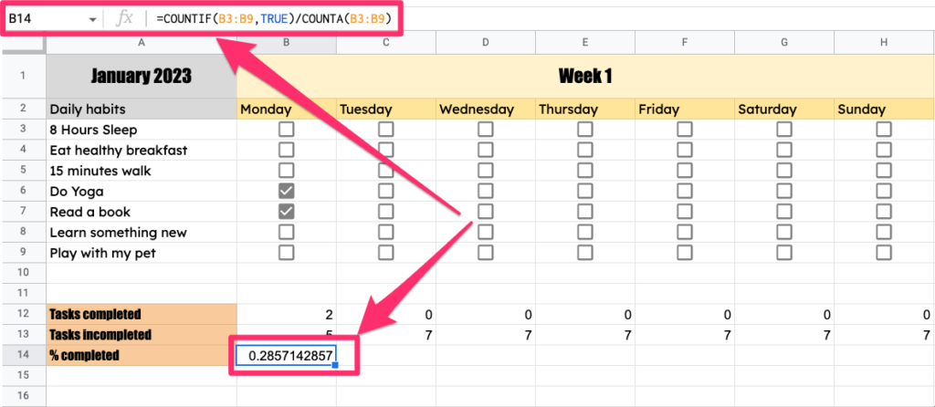
- The COUNTIF function will calculate all checkboxes that have the value set to TRUE
- The COUNTA function will simply count the number of cells in the provided dataset
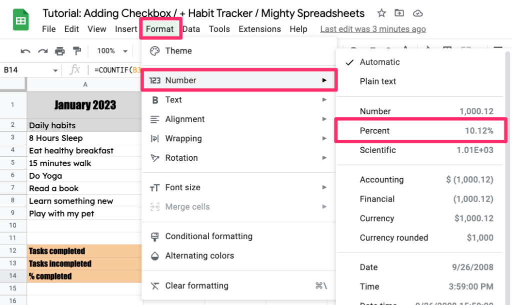
Now, all we need to do is change the number formatting to %. This is how to do it:
Step 8: While keeping your focus on the B14 cell navigate to Format > Number > Percentage Format in the Options menu
Step 10 (Optional): You can also add conditional formatting for your values.
If you want to do so go to “Format > Conditional formatting” and apply a few format rules.
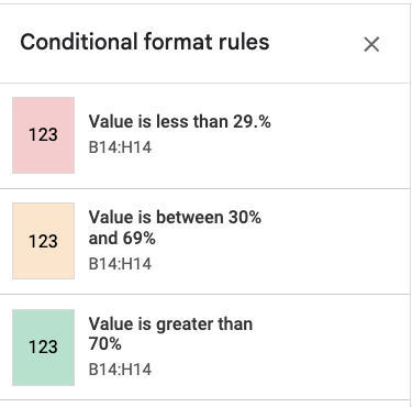
In this exercise, we will set 3 different colors depending on the cell value. In order to do that just select a “Color scale” option rather than “Single color“
- If the value is less than 30% then the cell will be highlighted in red
- If the value is between 31 and 69 then the cell will be highlighted in orange
- if the value is 70 or greater the cell will be highlighted in green
Here is the preview:
And this is the final effect:
Some Questions You May Have
Can I have multiple checkboxes in one cell?
No, you can’t have multiple checkboxes in one cell in Google Sheets. You will need to create separate checkboxes for each cell. Alternatively, you can use a drop-down menu that can have multiple values to pick from. All you need to do is to go to Data > Data Validation and pick “List of items” as your criteria (you need to provide the list too)
How do I delete a checkbox in Google Sheets?
To delete a checkbox from your sheet, just select the cells with the checkboxes and then hit the Delete key on your keyboard. This will remove any existing data validation rules as well as all values.
Is there a way to make a checkbox “checked” by default?
No, you can’t make a checkbox “checked” by default. The default value for the checkbox is unchecked and you can only change it manually by clicking on the checkbox itself.
My final thoughts
Checkboxes are a great way to quickly add interactivity to your Google Sheets. With this tutorial, you learned how to use checkboxes in Google Sheets in many different ways. Especially how to use formulas and conditional formatting with them.
I hope this guide was helpful! If you have any further questions or comments feel free to leave them in the comments section below. Thanks for reading and happy spreadsheeting!