This tutorial aims to give you detailed guidelines on how to round numbers in Google Sheets.
There are a few functions in Google Sheets that let you specify how to round numbers, and how many decimal places to display. There’s even a built-in function that will automatically format them if they are too long.
This is what we are going to cover in this article:
ROUNDfunctionROUNDUPfunctionROUNDDOWNfunction
This tutorial will take you approximately 5-10 minutes to complete. If you’d like to follow along feel free to make a copy of this sheet.
How to Round in Google Sheets (Google Sheets ROUND formula)
The ROUND function is the most straightforward Google Sheets function for this particular task.
The ROUND function rounds a number to a certain number of decimal places according to the rules you’ll provide.
The syntax for the ROUND function
The syntax for the ROUND function is pretty simple: ROUND(value, [places])
Where:
value– is the value you want to roundplaces– The number of decimal places to which to round. (An important thing to note is that if you don’t provide any argument, Google Sheets will use its default value of 0.)
NOTE: This function follows standard rules for rounding. It means that it considers the next most significant digit (the digit to the right) for performing the calculation. If this digit is greater than or equal to 5, the value is rounded up; otherwise, it’s rounded down.
Let’s have a look at some examples:
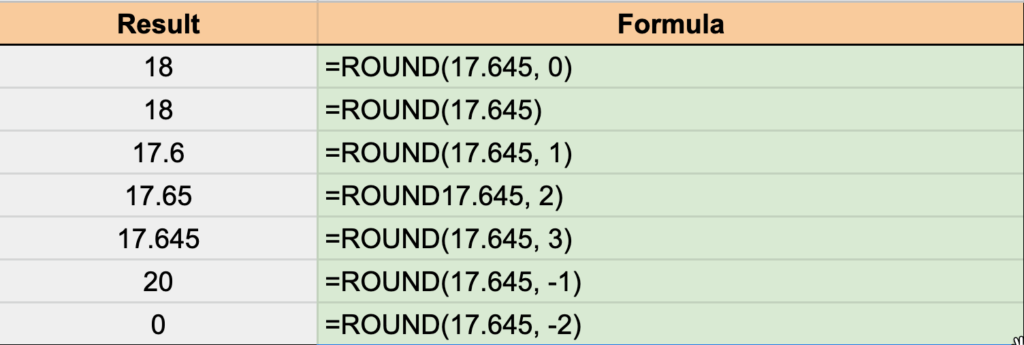
=ROUND(17.645)and=ROUND(17.645, 0)will be both rounded to the next whole number and the result will be 18 (remember when I mentioned that 0 is the default value for[places], right?)=ROUND(17.645, 1)will return 17.6 because we gave an instruction that we want 1 decimal place after the number=ROUND(17.645, 2)will round to 2 decimal places and return 17.65, and so on. It should be pretty straightforward to follow.
Now that you know how to round decimals in google sheets let’s talk about something different.
How To Use Google Sheets Round Function With Negative Values
The thing you may not be aware of is that you can also use negative numbers as a places argument.
Round the value up or down to the nearest 10
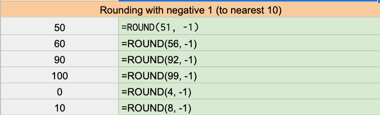
If you want to round your value to the nearest ten, then you simply need to provide -1 as the places argument. A few examples:
=ROUND(51, -1)will return 50=ROUND(56, -1)will return 60=ROUND(92, -1)will return 90=ROUND(99, -1)will return 100=ROUND(4, -1)will return 0=ROUND(8, -1)will return 10
Round the value to the nearest 100
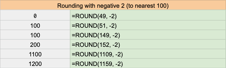
If you want to round your value to the nearest hundred, use -2 as the places argument.
Here are a few examples so you can put it into practice:
=ROUND(49, -2)will return 0=ROUND(51, -2)will return 100=ROUND(149, -2)will return 100=ROUND(152, -2)will return 200=ROUND(1109, -2)will return 1100=ROUND(1159, -2)will return 1200
Round the value to the nearest 1000
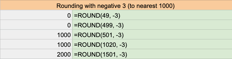
For numbers that you want to round to the nearest thousand, use -3 as the places argument. A few examples:
=ROUND(49, -3)will return 0=ROUND(499, -3)will return 0=ROUND(501, -3)will return 1000=ROUND(1020, -3)will return 1000=ROUND(1501, -3)will return 2000
Alright, Now that you understand how the ROUND function works (with some edge cases included).
However, there may be a time when you always want a number to be rounded up or rounded down. In the next chapters, we will cover this topic in more detail.
How to Round Up in Google Sheets
The ROUNDUP function always rounds a value upward. For example, if you wanted to round up to the nearest 1 or nearest 10 or nearest 100 this function would allow Google Sheets to do that for you.
The syntax for the ROUNDUP function is pretty simple: ROUNDUP(value, [places])
Let’s have a look at a few examples:
- both
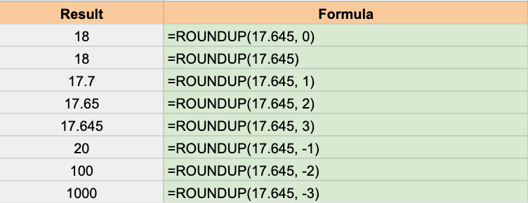
=ROUNDUP(17.645)and=ROUNDUP(17.645, 0)will round up to the nearest whole number and the result will be 18 =ROUNDUP(17.645, 1)will round up to the nearest decimal place and the result will be 17.7=ROUNDUP(17.645, 2)will round up to the nearest two decimal places and the result will be 17.65=ROUNDUP(17.645, 3)will round up to the nearest three decimal places the result will be 17.645=ROUNDUP(17.645, -1)will round up to the nearest 10 and the result will be 20=ROUNDUP(17.645, -2)will round up to the nearest 100 and the result will be 100=ROUNDUP(17.645, -3)will round up to the nearest 1000 and the result will be 1000
I guess it should be pretty straightforward for you now. On the other side if you always want to have the numbers rounded down then you should the ROUNDDOWN function.
How to Round Down in Google Sheets
The ROUNDDOWN function always rounds a value downward. The function enables Google Sheets to round down numbers to the nearest unit you specify, such as 1, 10, or 100.
The syntax for the ROUNDDOWN function is exactly the same: ROUNDDOWN(value, [places])
A few examples below will help you understand how the function works:
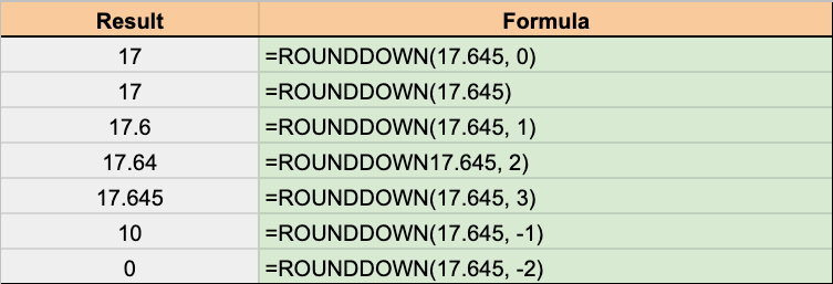
=ROUNDDOWN(17.645, 0)will return 17=ROUNDDOWN(17.645)will return 17=ROUNDDOWN(17.645, 1)will return 17.6=ROUNDDOWN17.645, 2)will return 17.64=ROUNDDOWN(17.645, 3)will return 17.645=ROUNDDOWN(17.645, -1)will return 10=ROUNDDOWN(17.645, -2)will return 0
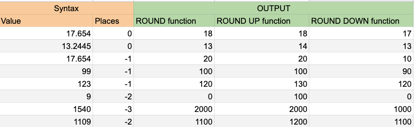
Rounding in Google Sheets – birds-eye view comparison
To wrap up this Google Sheets rounding tutorial, here is a screenshot of a table that provides you with an easy to compare the birds-eye view of ROUND vs. ROUNDUP vs. ROUNDDOWN functions:
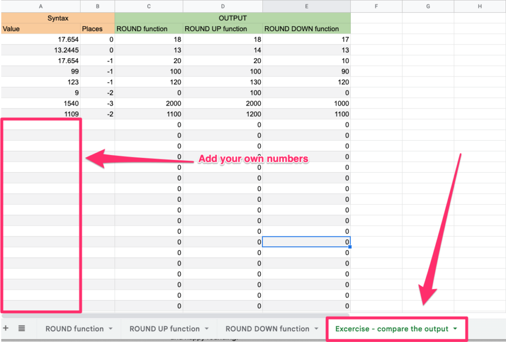
If you’d like to experiment with your own numbers you can do it in the “Excercise – compare the output” worksheet that I prepared in the training material (you can copy it here if you haven’t already)
My final thoughts
Now you have a better understanding of how to round numbers in Google Sheets. Rounding is an important skill to have when working with data. The ROUND, ROUNDUP, and ROUNDDOWN functions are three versatile tools that can be used to get your numbers into the format that you need.
I hope you found this tutorial helpful and now feel more confident about using the rounding functions in Google Sheets.
If you have any questions or comments, please let me know in the comment section below. Good luck and happy rounding!