How to Hide and Unhide Rows and Columns in Google Sheets

This article aims to give you an ultimate guide on how to hide and how show hidden rows and columns in Google Sheets.

We go over many different ways of hiding, showing, and finding cells that are hidden. We’ll cover this ground for both desktop and mobile applications. Furthermore, I’ll include some tips on how to debug the most common issues people face during the process.

How to Hide Rows In Google Sheets

Hiding rows is a very convenient way to compare some data without any distractors. It’s super easy to hide any row in Google Sheets. Here’s what you need to do:

Step 1: Select a row or rows that you want to hide by simply clicking on the row number.

Here are some things worth noticing:

• If you want to select multiple rows press and hold the SHIFT key and click on the first and last row of your selection or simply hold your left mouse button clicked and drag your mouse down.

• If you want to select multiple rows that are not close to each other then just click on them having the CTRL (Windows) or COMMAND (Mac) key pressed

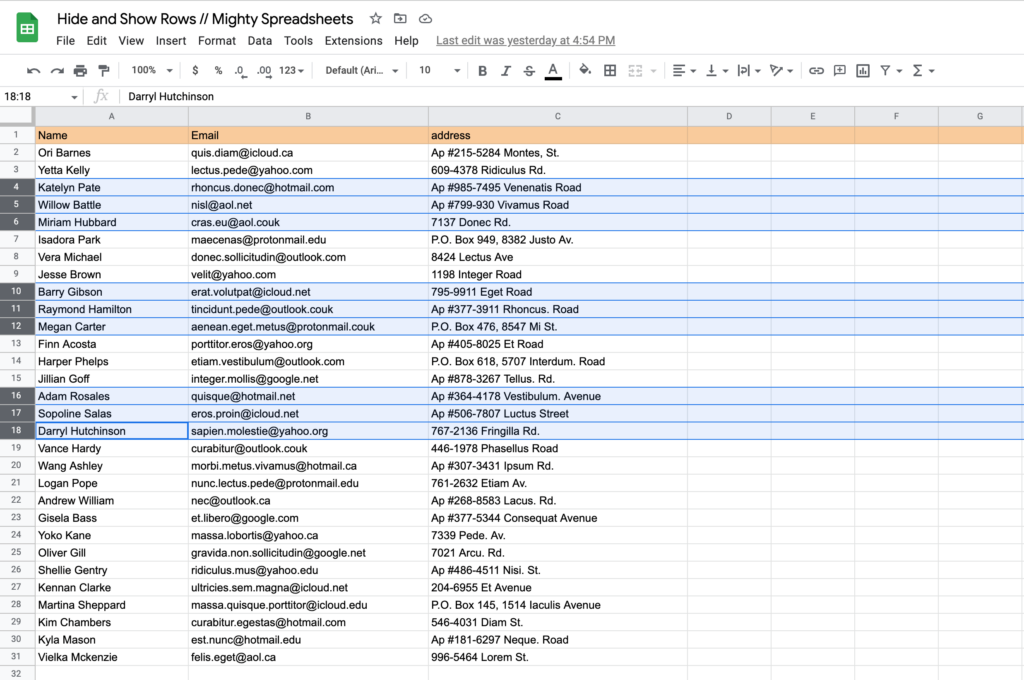
This is the output you should expect:

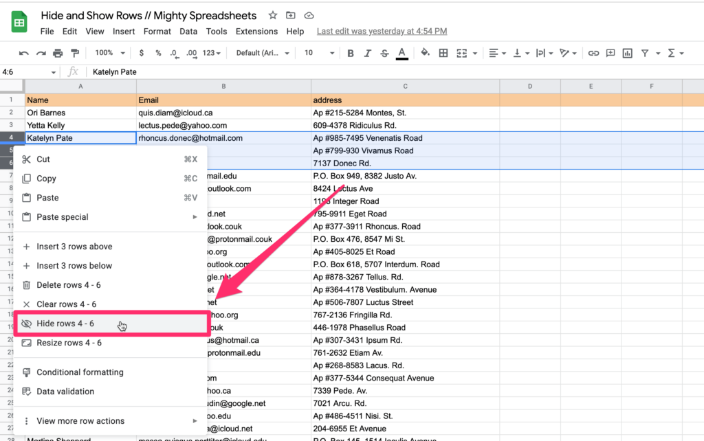
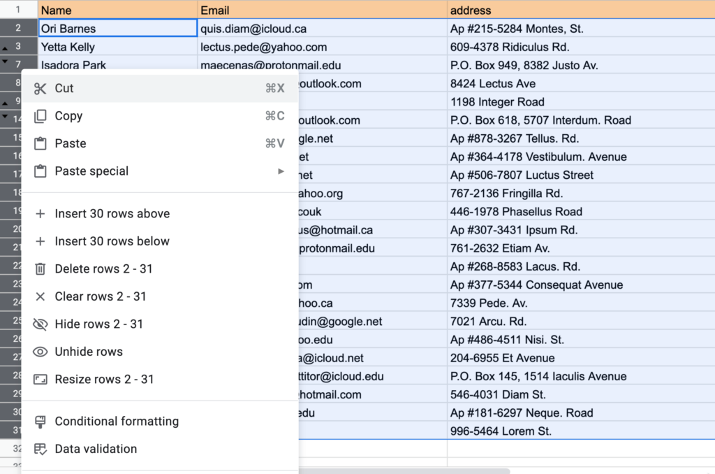
Step 2: Right-click on the selection

Step 3: From the popup menu that will appear select the “hide rows” option

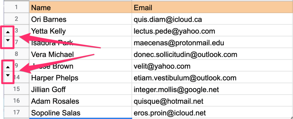
Step 4: Observe that rows are hidden and there are two arrows indicating that fact

Alternatively, you can also achieve the same result using the keyboard shortcut after you select your rows:

• Press COMMAND + OPTION + 9 to hide rows if you are on Mac
• Press ALT + CONTROL + 9 to hide rows if you are on Windows

Now that we know how to hide rows let’s have a look at possible ways of showing the missing rows back.

How to Unhide Rows in Google Sheets

#1: Unhide rows using the arrows

It’s probably the best option to use if you don’t have many rows hidden. Just click on one of the arrows that appeared when you were hiding the rows and you are done.

#2: Unhide rows using the contextual menu

You can show hidden rows by selecting all the rows you want to unhide and clicking on the selection with your right mouse button.

The simplest way to select more than one row that isn’t adjacent to each other is by holding down the CTRL/COMMAND key and clicking on the rows you want to select with your left mouse button.

Here’s what the process looks like:

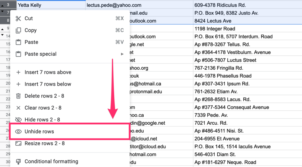
Step 1: Select the range of hidden rows

Step 2: Right-click on the selected range and select the “Unhide rows” option from the popup that appeared

This works best when you have a moderate number of hidden rows and don’t need to reveal all of them at once.

#3: how to unhide all rows in google sheets

I wish I could just say that you can select the entire worksheet and click on “Unhide rows” but that’s unfortunately not true.

What you can do though is to select a wider range of cells manually and unhide rows then. These are the steps you should cover:

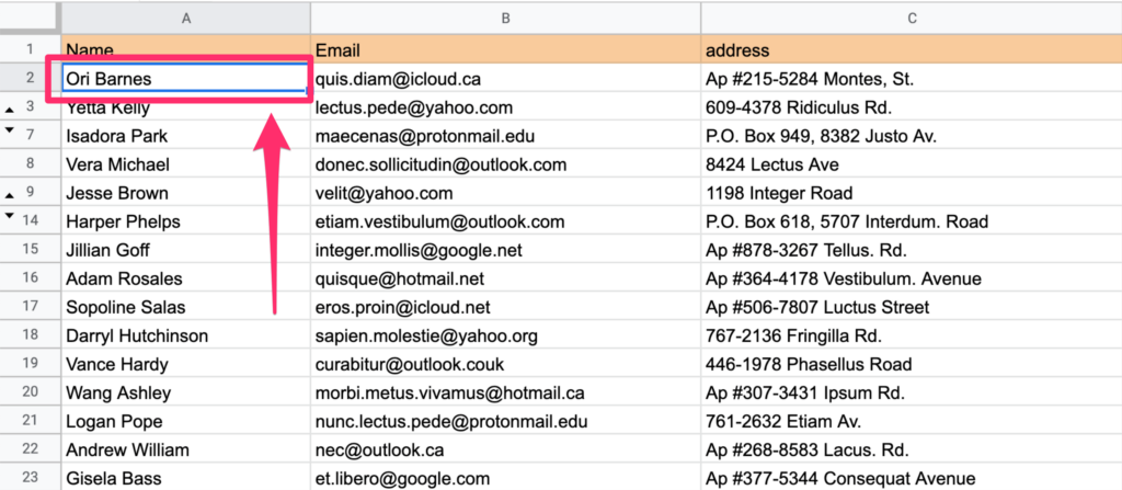
Step 1: Focus on the first cell on top of your selection (in this example it’s going to be the A2 cell)

Step 2: Hold the SHIFT key and click on the row that is going to be the last item in your selection

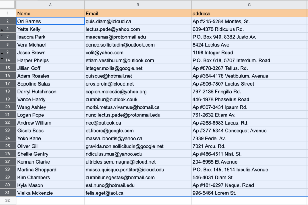
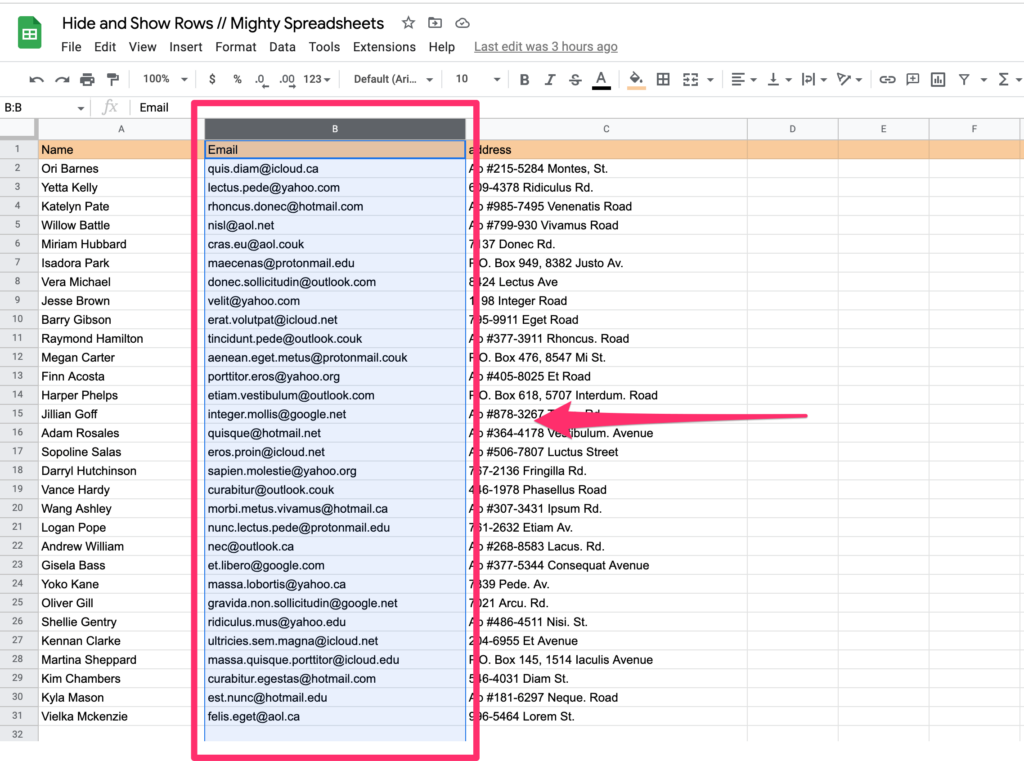
Step 3: Right-click somewhere on selected rows and select the “Unhide rows” menu item.

How to unhide rows hidden by a filter

There’s one more thing that I think we should cover. In some cases, rows may appear as hidden but they are actually only filtered out.

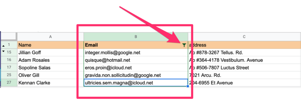
The easiest way to notice that is by looking at the columns. The one that has a filter applied to it will have a light green background on the column heading and a blue filter icon on the column header.

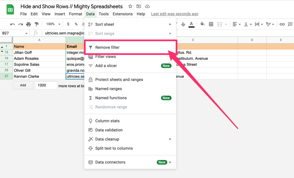
The easiest way to get rid of those filters is through the Options Menu. Just navigate to the “Data” menu item and pick “Remove filters”. This should get the job done for you.

How to hide columns in Google Sheets

Hiding columns is as easy as hiding rows.

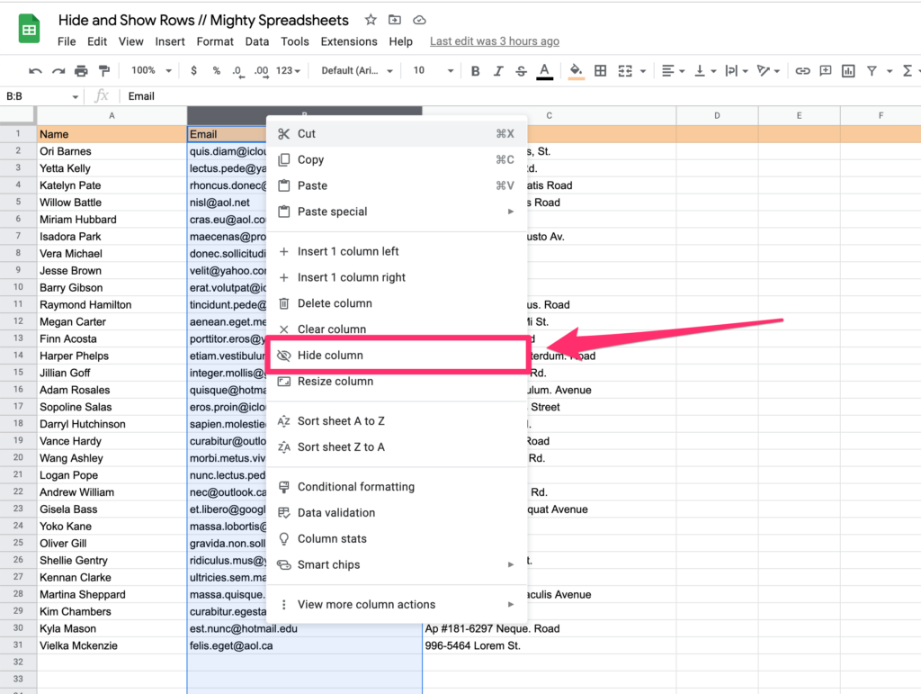
Step 1: Select the Column you wish to hide

Step 2: Right-click on it

Step 3: Select the “hide columns” option from the contextual menu that will appear.

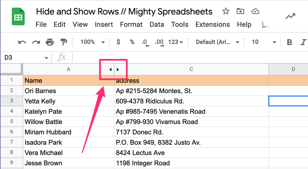
You will notice the horizontal arrows appearing next to the hidden column.

You can also achieve the same outcome by using this keyboard shortcut after you select your columns:

• Press COMMAND + OPTION + 0 to hide columns if you are on Mac
• Press ALT + CONTROL + 0 to hide columns if you are on Windows

By understanding how to hide columns, we can now explore ways of showing the missing columns again.

How to unhide columns in Google Sheets

#1: Unhide columns by clicking on the arrows

If you don’t have many hidden columns, this is probably the best option. To use it, just click on one of the arrows that appear when you hide a column.

#2: Unhide columns using the contextual menu

To unhide hidden columns, select the ones you want to view and click on the selection with your right mouse button.

To select more than one column that isn’t next to each other, hold down the CTRL/COMMAND key and click on the columns you want to select with your left mouse button.

Here’s what it’s going to look like:

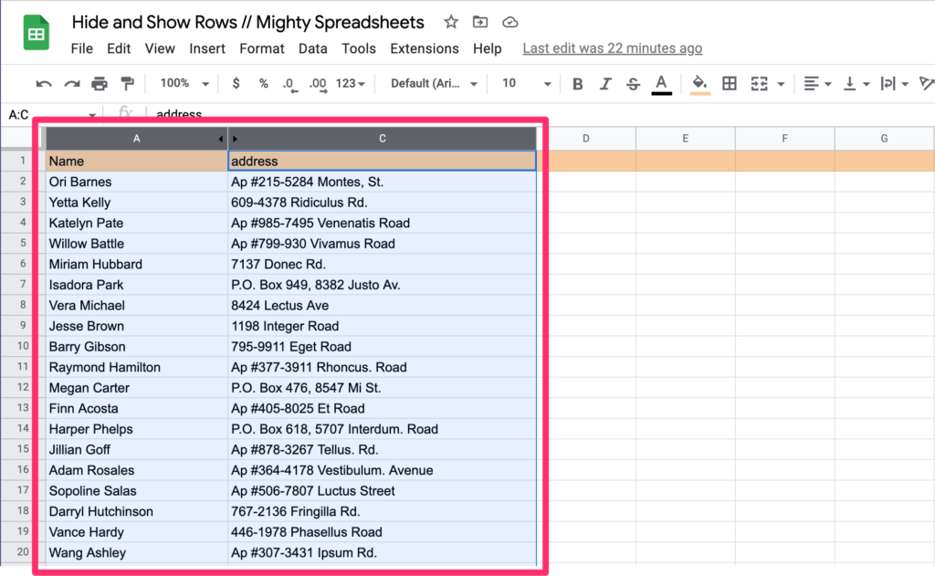
Step 1: Select the range of hidden columns

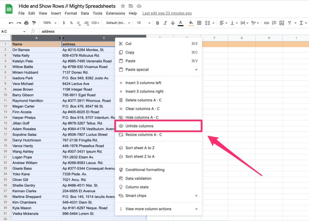
Step 2: Right-click on the selected range and select the “Unhide columns” option from the popup that appeared

#3: how to unhide all columns in google sheets

If you want to unhide a wider selection of columns these are the steps you should go through:

Step 1: Focus on the first cell on top of your selection (in this example it’s going to be the A1 cell)

Step 2: While holding SHIFT, click on the column that is going to be last in your selection.

Step 3: Right-click somewhere on selected columns and select the “Unhide columns” menu item.

How to Hide Rows in Google Sheets Mobile App (iPhone,iPad, Android)

Although hiding rows on the mobile app looks different than doing it on a desktop, it’s actually just as easy:

Step 1: Select the row or rows that you want to hide

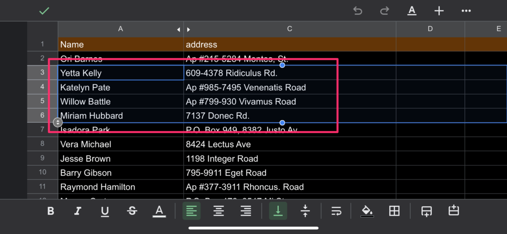
The blue drag icon is located around the focused cell and allows you to select more than one row if needed. To do this, simply tap on it and extend your selection.

Step 2: Double-click on the selected range and find the “Hide rows” option in the contextual menu

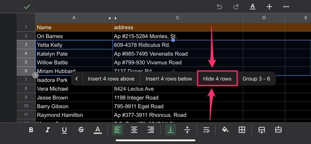
Simple as that.

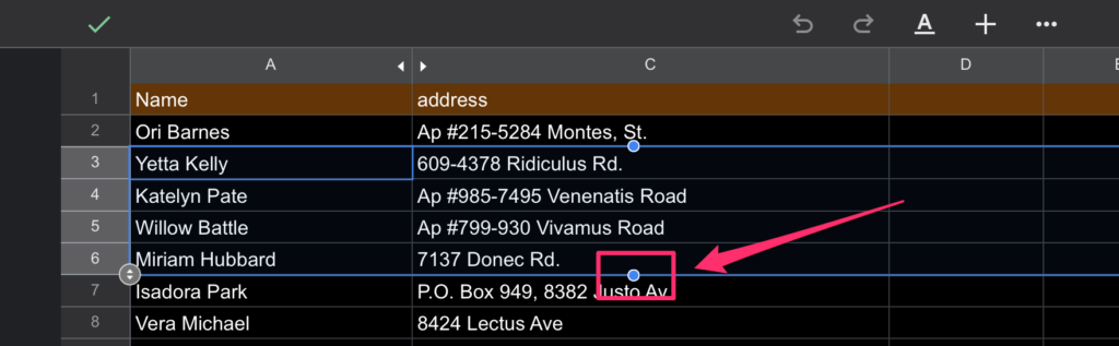
If you want to show your rows again, just tap on the arrows that appear after you’ve hidden them.

Note: The process of hiding/showing columns in the mobile app is exactly the same, you just need to select columns instead of rows.

Some Questions You May Still Have

Summary

Knowing how to hide rows or columns can provide you with more efficient ways of navigating your spreadsheets and comparing the data.

The process of hiding them is fairly easy, as you’ve seen here. You just need to select the rows or columns and use the contextual menu to find the “Hide” option.

To unhide them, you can use the arrows that appear after they’re hidden or by using the contextual menu.

Finally, if the option to unhide rows is not working it’s likely because they’re hidden with a filter. You can get rid of those filters through the Options Menu.