You can add hyperlinks in Google sheets to quickly access external web pages, another sheet in Google sheets, or even a cell in the sheet itself.
The simplest way to add a hyperlink in Google Sheets is to select the cell and click on the “insert link” button on the toolbar. This will open up the link options. Paste the link and click apply and that’s it!
In this post, I’ll give you a detailed breakdown of how to hyperlink in Google sheets along with a few useful ways of using hyperlinks in various use cases.
How To Create Hyperlink In Google Sheets
There are 4 ways to hyperlink in Google sheets:
- Keyboard shortcut,
- The toolbar shortcut,
- Options menu,
- The hyperlink formula.
1. Create a Hyperlink Using Keyboard Shortcut
This is my favorite method of adding a hyperlink because it’s super fast. If you are like me and you prefer using shortcut keys to increase productivity, then you can use:
- Ctrl + K is the hotkey on Windows,
- Cmd + K is the hotkey for Mac
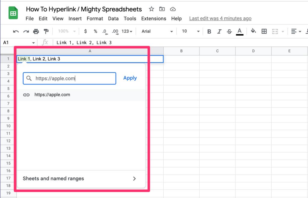
You will see a dialog box popping up:
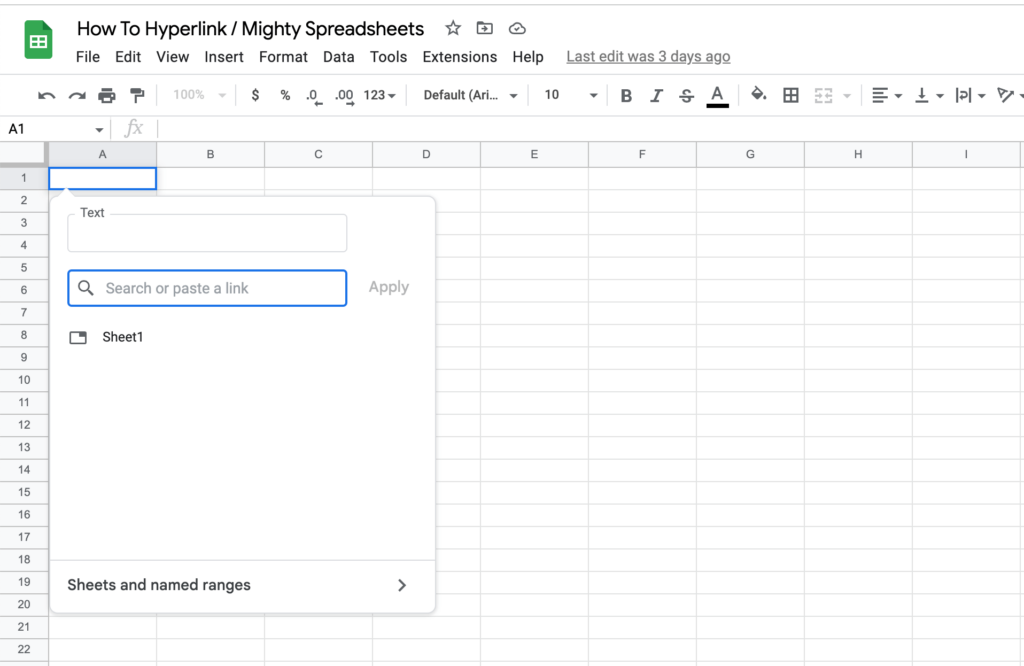
The next steps are the following:
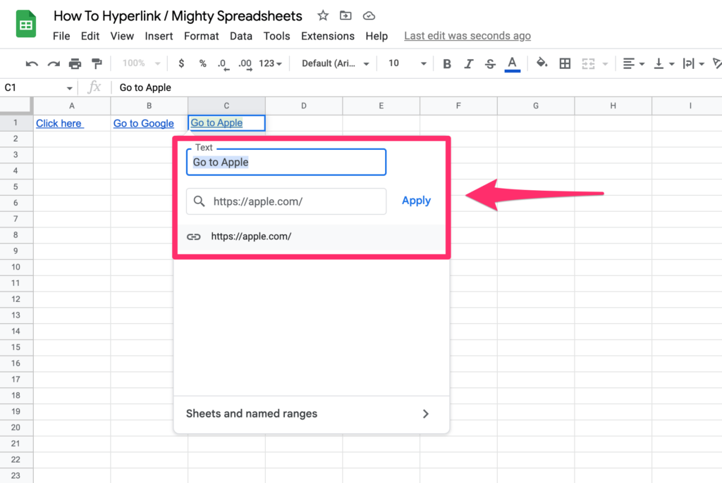
Step 1: Insert the URL you want to be your link anchor
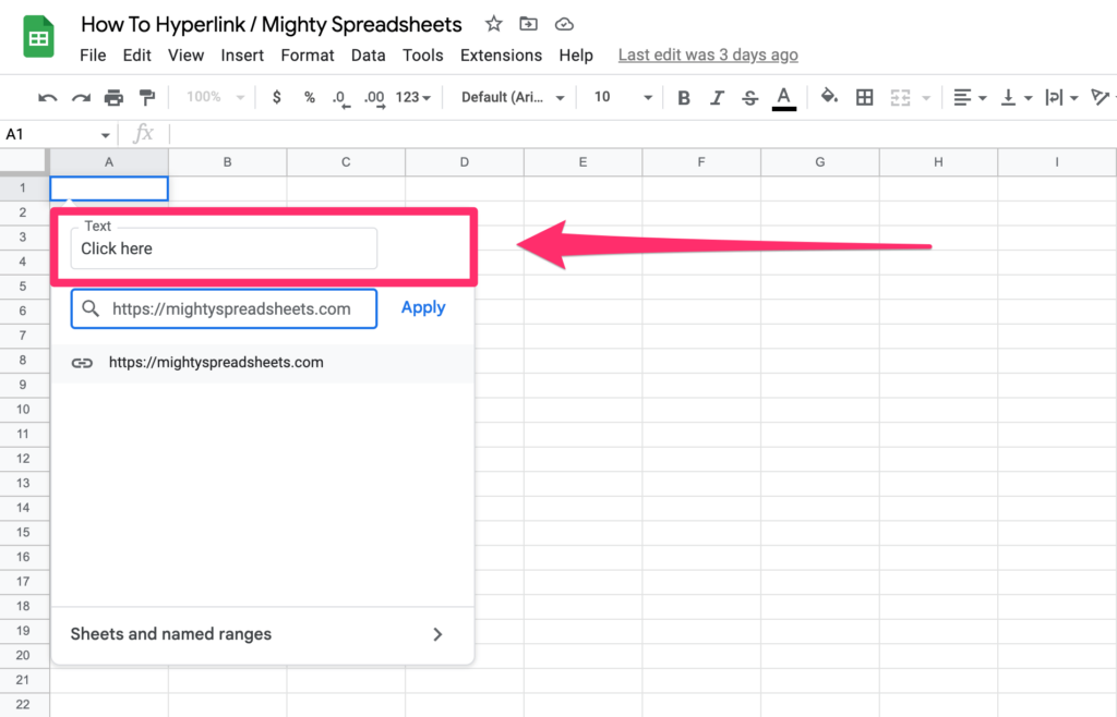
Step 2: Insert the web address you want to create a hyperlink to in the text box.
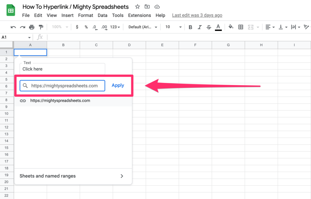
Step 3: Click on apply or hit Enter to create the hyperlink.
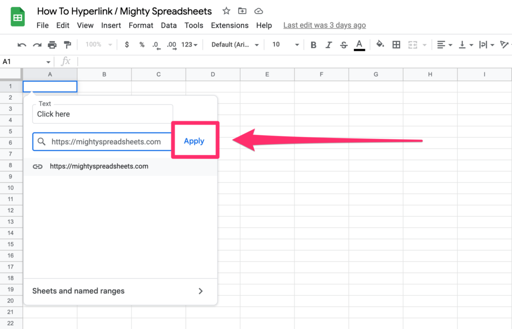
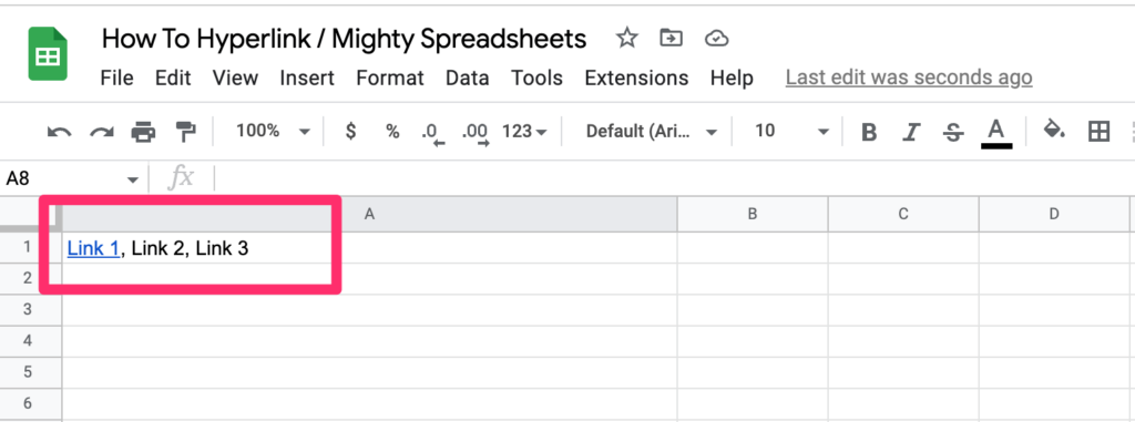
Now you can see that the text in the cell turned blue and underlined, indicating it is a link.
To edit or remove the hyperlink, click on the cell and select Edit link or Remove link from the options that appear below the hyperlink.
2. Add Hyperlink Using the Toolbar Shortcut
Using the toolbar shortcut is pretty straightforward and will be a great solution in many cases so let’s explore it now:
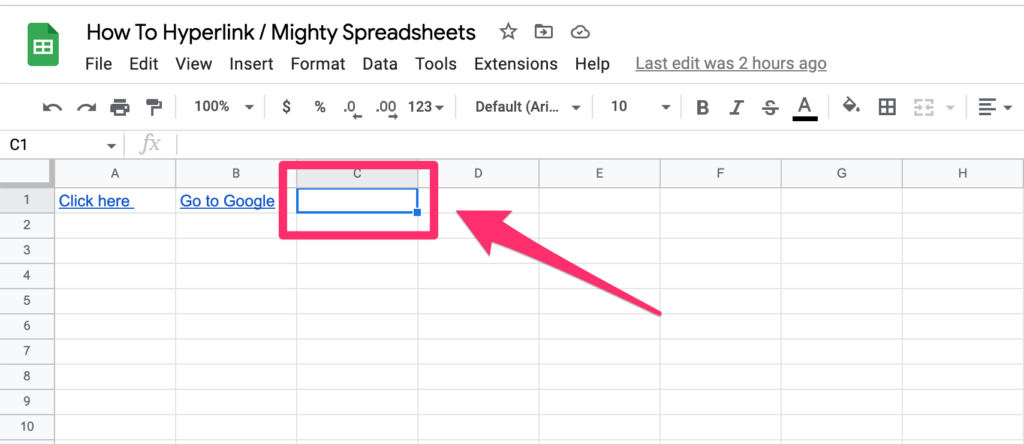
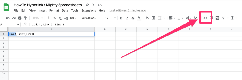
Step 1: Focus on the cell where you want to add a hyperlink
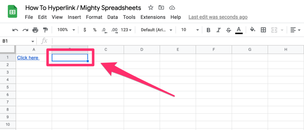
Step 2: Click on the Hyperlink icon
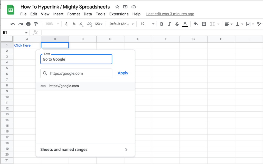
Step 3: Fill the popup with anchor text and your link and click Apply
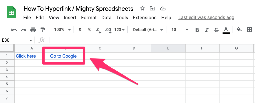
Easy peasy lemon squeezy! You just created a hyperlink using a toolbar icon and this is how the final effect looks like:
Now let’s take a look at the other options in greater detail.
3. Use the Options Menu To Create a Hyperlink
To create a clickable link in Google sheet using the options menu, you need to follow these steps:
Step 1: Select the cell you want to the hyperlink.
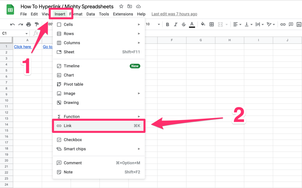
Step 2: Select “Insert” from the Options Menu, then just click on the “Link” option, and a small dialog box will show up.
Step 3: Provide anchor text and the URL for the link
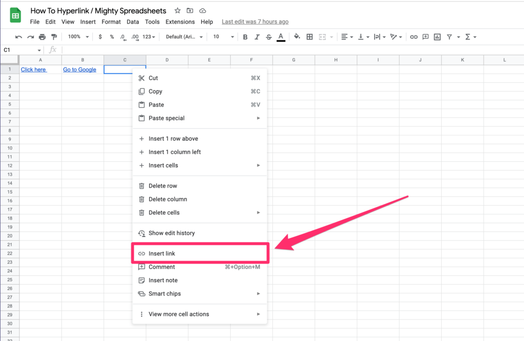
Quick Tip – You can quickly access this option by right-clicking on the cell and selecting the Insert link option from the menu 👇👇👇
4. Use Google Sheets Hyperlink Formula
Using the formula method to create a hyperlink is a little bit more complicated than using the options menu. But it is worth knowing how to do so.
You can create a hyperlink with a simple syntax in Google sheets.
=HYPERLINK(“URL”, “TEXT”)
URL– The link to the web address that needs to be inserted as the hyperlink. It should be enclosed within double quotes.
TEXT– The text that needs to be shown in the cell. This too must be placed in double quotes.
- The
URLandTEXTvalues are separated by a comma.
Have a look at the example below:
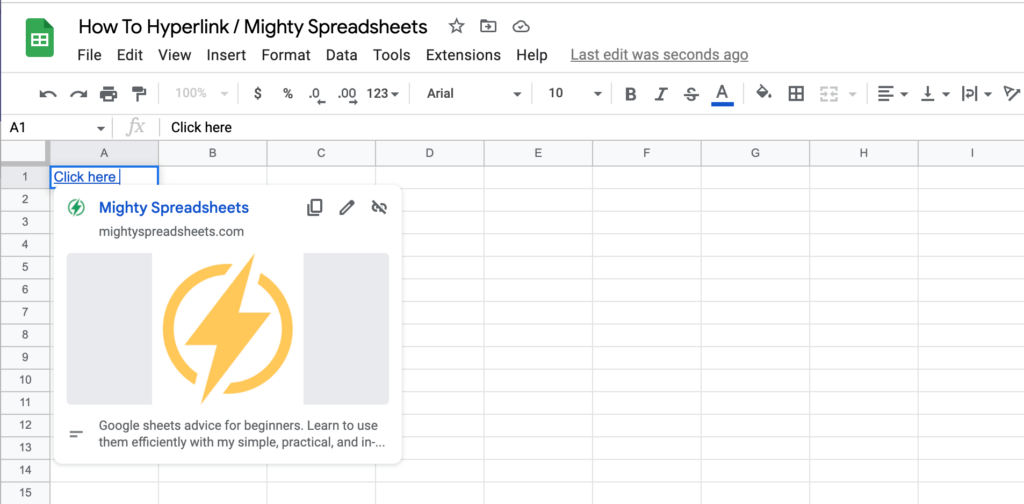
=HYPERLINK("http://mightyspreadsheets.com", "Mighty Spreadsheets")
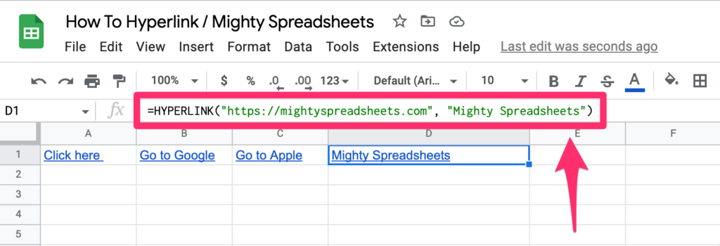
Once clicked or hovered over the cell, the link is shown in a small popup box. The web page will open in a new tab after clicking on the link.
5 Different Ways To Use Hyperlinks
1. Hyperlink To Another Sheet In Google Sheets
We can create hyperlinks between sheets in the same document in Google sheets. This is very useful when you are managing several sheets in a single document.
To add a clickable link to another sheet in Google sheets follow these steps:
Step 1: Select the cell in which you want to insert the hyperlink.
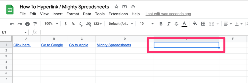
Step 2: Get the Insert link dialog box by using any of the methods we talked about earlier
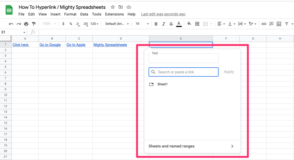
Step 3: In the dialog box, click on ‘Sheets and named ranges’.
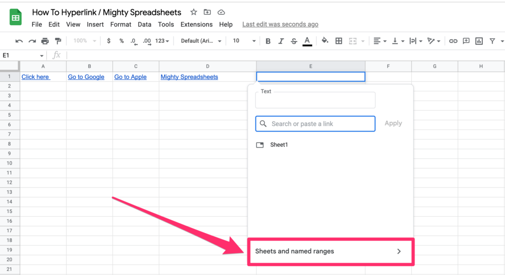
Step 4: A list of available sheets in the document will appear. Select the sheet which you want to link.
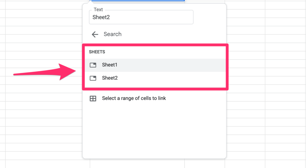
Step 5: Click on Apply or hit enter to create the hyperlink.
Now when you click on the hyperlink it will automatically open the worksheet you linked to:
2. Hyperlink To A Cell or a Named Range In Google Sheets
Creating a hyperlink to a cell or a cell range in Google sheets is pretty similar to linking another sheet.
To add hyperlinks to a cell range in Google sheets:
Step 1: Select the cell and get the Insert link dialog box
Step 2: In the dialog box, click on ‘Sheets and named ranges’. There is an option as ‘Select a range of cells to link’ below the sheets. Click on it.
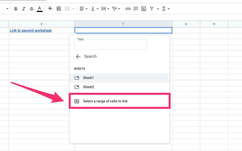
Step 3: A text box will appear.
- If you want to link a single cell, Insert the cell’s reference. (Example:
B25) - To link a range of cells, insert the first and last cell numbers separated by a colon (Example:
E4:H8) - You can also link to a named range of cells if you previously created one
Step 4: Click on Apply or hit enter to create the hyperlink.
3. Add Hyperlink To A Url In Google Sheets
You can also use hyperlinks to direct someone to an external website from Google sheets.
So how to paste a link in google sheets? Simply, we already covered it at the beginning of this article:
Step 1: Select the cell and get the Insert link dialog box.
Step 2: In the textbox, type or paste the URL you want to add as a hyperlink. Click Apply.
Clicking on these hyperlinks will open the web page in a new tab.
4. Add Dynamic Hyperlink In Google Sheets
Dynamic hyperlinks are links that change based on cell values.
Dynamic hyperlinks should be created using the formula we talked about earlier.
To create a dynamic hyperlink using the HYPERLINK function we have to insert the sheet name and the cell reference followed by a hash symbol (#). So, the generic version of the formula will be
=HYPERLINK(“URL“&CELL_REFERENCE,“CELL_TEXT”)
CELL_REFERENCE– The reference (ID) of the cell where your link needs to get the data.CELL_TEXT– The text that needs to be shown in the cell.
Let’s take a look at a real-life example to get a better idea:
=HYPERLINK("https://apple.com/"&G2, "Link")
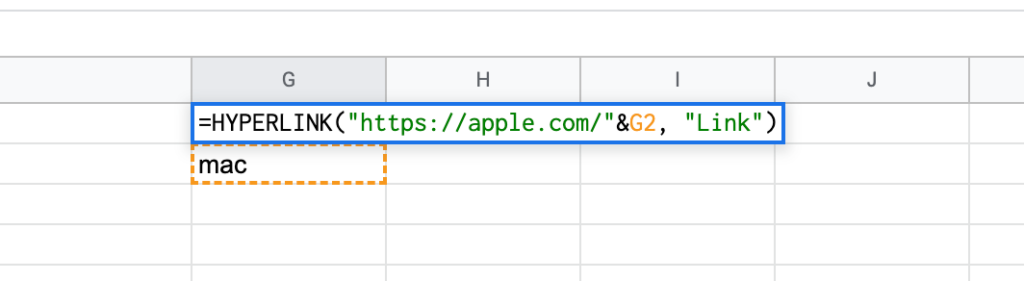
Depending on the value of the G2 cells you will be redirected to different pages. For example, if the G2 cell value was “mac” you would be redirected to “https://apple.com/mac” if the value of the G2 cell was “iphone” you would be redirected to “https://apple.com/iphone“
5. Add Hyperlink To Send An Email In Google Sheets
You can add hyperlinks to send an email by either the Insert link method or the formula method.
The insert link method is easier but the formula method comes in handy with more options such as creating a hyperlink to multiple email addresses at once.
Using the Insert link method:
- Select the cell and get the Insert link dialog box.
- In the textbox, type “mailto:” and then insert the email address you want to add as a clickable link in google sheets and click apply.
Using the formula method:
You can use the below syntax to create a hyperlink in Google sheets.
=HYPERLINK("mailto:EMAIL_ADDRESS","CELL_TEXT")
EMAIL_ADDRESS– The email address to which you want to send an email.CELL_TEXT– The text that needs to be shown in the cell.
For example,
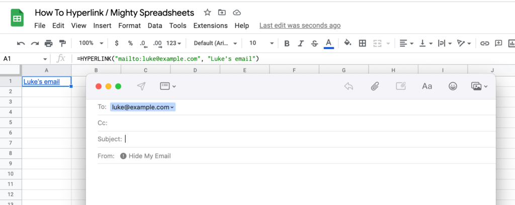
=HYPERLINK(“mailto:[email protected]“, “Luke’s email”)
How To Edit Hyperlink In Google Sheets
To edit a hyperlink in Google sheets,
Step 1: Click on the cell where you created the hyperlink.
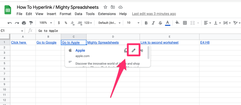
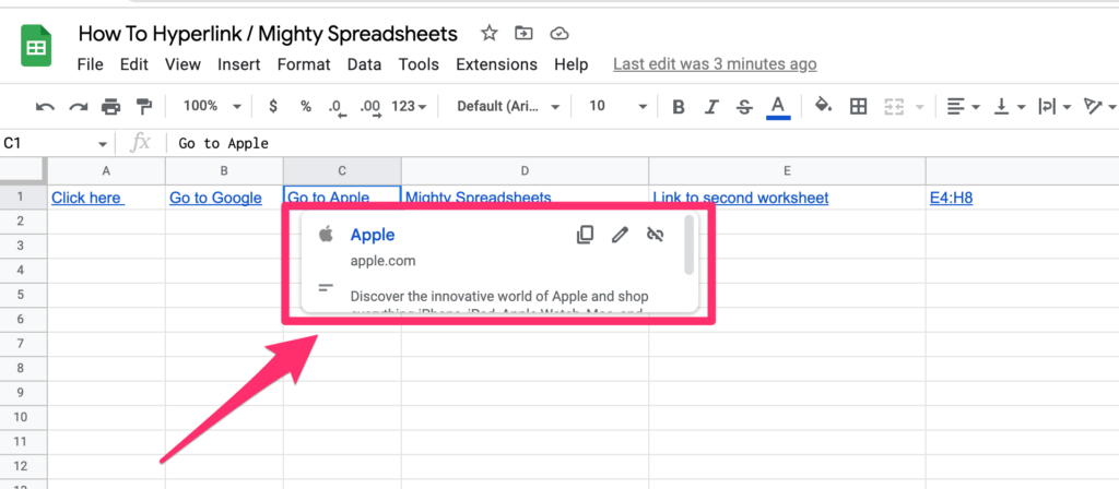
Step 2: A small popup box will appear which shows the link that it contains. There are 3 icons next to the link.

Step 3: Click on the pencil icon in the middle to edit the hyperlink. It will show the dialog box which we use to create the hyperlink.
Step 4: Edit the details and click on Apply button to save the changes.
How to Remove Hyperlink in Google Sheets
To remove a hyperlink in Google sheets,
Step 1: Click the hyperlinked cell.
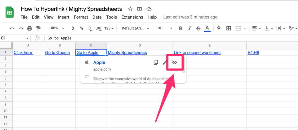
Step 2: A small popup box will appear which shows the link that it contains. There are 3 icons next to the link.
Step 3: Click on the third icon to remove the hyperlink.
How Do I Create A Hyperlink In The Google Sheets Mobile App?
Creating a hyperlink in the Google Sheets mobile app is pretty similar to the desktop version there are however some minor differences between Android and IOS devices.
How to Create a Hyperlink in iPhone / Ipad Google Sheets mobile App?
At the time of writing this article, there’s no way to add a hyperlink from the Options menu in the IOS app. Here’s what you need to do if you want to add it on your phone (or tablet):
Step 1: Open the document and tap to select the cell that you want to create a hyperlink.
Step 2: Use the hyperlink formula to add your link.
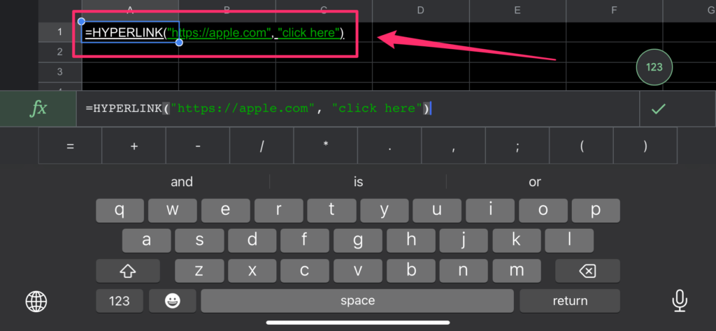
For example:
=HYPERLINK(“https://apple.com/”, “Click here”)
Step 3: Apply your formula by clicking on the tick icon
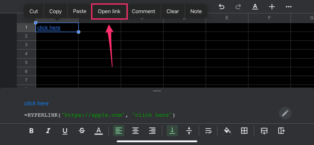
Note: When you click on the link it won’t open automatically. You will need to select “Open link” from the contextual menu
How to Create a Hyperlink in Android App?
Step 1: Open the document and tap to select the cell that you want to create a hyperlink.
Step 2: Click on the + sign next to the cell or the Insert option from the top menu. (This may depend on your device and the app version)
Step 3: From the drop-down menu that appears, select the Link option to add a hyperlink.
Step 4: Paste or insert the URL you want to add and a text to show in the cell.
Some Other Questions You May Have
How Do I Put Multiple Hyperlinks In One Cell In Google Sheets?
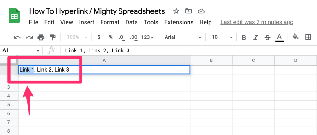
You can put hyperlinks to multiple words in the same cell using Google sheets.
The only difference is, you should select the word or words using the mouse pointer instead of just selecting the whole cell.
Step 1: Select the word(s) you need to add a hyperlink.
Step 2: Select the Link option from the insert menu or the Insert link option from the right-click menu.
Step 3: Insert the link address and click on apply or hit enter to create the hyperlink.
And this is the final effect:
You can repeat the process to add hyperlinks to other words.
Why Is My Google Sheets Link Not Working?
There can be a couple of reasons why hyperlinks are not working. First, check whether you have entered the link address correctly. If you copied the link from someplace, see if you copied the full link without missing any letters.
It could also be that the linked website might be down or changed to another URL. Try accessing the link using a browser to check if there is something wrong with the web page.
If you are creating the hyperlink using the formula method, thoroughly check whether you are doing it with the correct syntax. A single mistake will cause the hyperlink to not work.
Can You Hyperlink An Image In Google Sheets?
You can hyperlink an image in Google Sheets, however, it is a little bit more tricky than using text. But don’t worry, I’ll break it down step by step on how to hyperlink an image in Google Sheets.
First up, your image must be on the internet to copy the URL.
For example, you can get it from an external website (such as Pexels)
Adding a hyperlink to an image should be done with the formula method I explained earlier. This is achieved by including the IMAGE function with the HYPERLINK function in Google sheets.
Get an image from the internet as the hyperlink image
Follow the below syntax to add a hyperlink to an image.
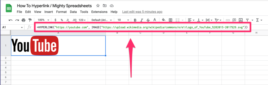
=HYPERLINK(“URL”, IMAGE(“IMAGE_URL”))
URL– The link to the web address that needs to be inserted as the hyperlink.IMAGE_URL– Web link of the image you want to create the hyperlink.
Example hyperlink formula to get a better idea:
=HYPERLINK("https://youtube.com", IMAGE("https://upload.wikimedia.org/wikipedia/commons/e/e1/Logo_of_YouTube_%282015-2017%29.svg"))
Google sheets will automatically insert the image from IMAGE_URL you provide and create the hyperlink with the URL.
Get Your Own Image As the Hyperlink Image
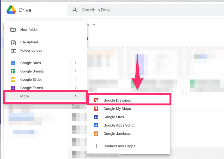
To have an image from your local PC or Google Drive as the hyperlink image, first, you should upload it as a Google drawing.
Step 1: Go to your Google Drive, Click on New, and select Google Drawings from the drop-down menu. (or you can go directly to Google Drawings by clicking on this link)
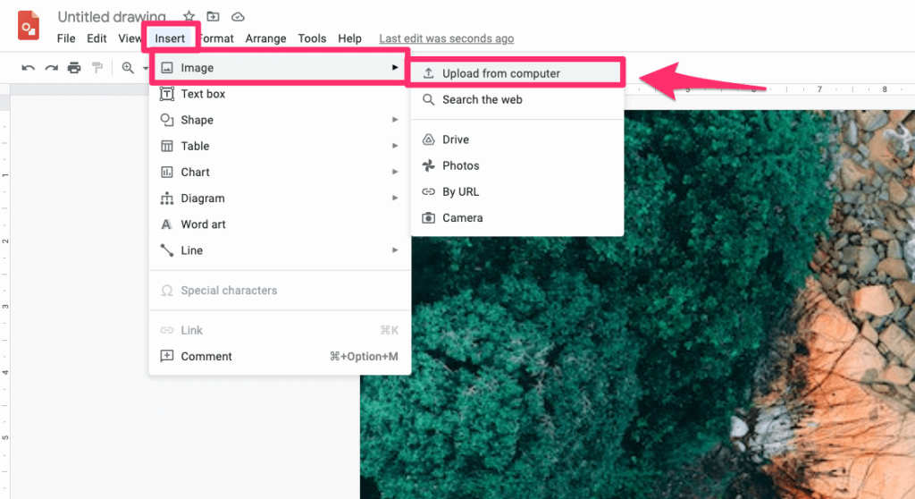
Step 2: Click on:
- “Insert” menu item from the top menu,
- then on the “Image” sub-menu item
- finally, select “Upload from computer“.
Step 3: Now you can upload the image from your PC or Google drive by browsing the files. Or else, simply drag and drop the image onto the blank drawing sheet.
Step 4: Adjust the image as you like. Remove any unwanted margins to give the hyperlink a better look.
Now the image is ready and we have to publish it to the Web in order to get the URL.
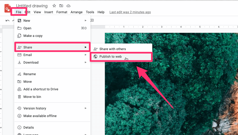
Step 5: Click on the File menu item and select Publish to Web option under the Sharing section.
Step 6: Make sure you have selected the Link tab and resize the image size (you can pick from 3 options: small, large, or medium.
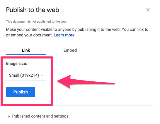
Step 7: Click on the Publish button and now you will see a link is created for the image.
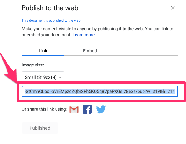
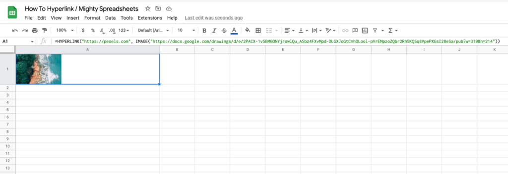
Simply copy the link and insert it as the IMAGE_URL. Here is the syntax in case you forgot how to create a hyperlink using the formula.
=HYPERLINK(“URL”, IMAGE(“IMAGE_URL”))
Now you’ll see the image is inserted in the cell. Click on it to see the hyperlink which has been created.
How to Hyperlink a PDF in Google Sheets?
We can create a hyperlink to documents such as PDF files in Google sheets. When someone clicks on the hyperlink, the file will be downloaded instantly.
This is another very useful feature in Google sheets when you want to share PDF files in an organized manner.
Step 1: In order to share a PDF, first you need to upload it to Google drive.
Step 2: Then right-click on the PDF file and select the get link option. If you don’t see such an option, go to Share and click on the get link button at the bottom. Make sure you have selected access to ‘Anyone with the link’ instead of the ‘Restricted’ option.
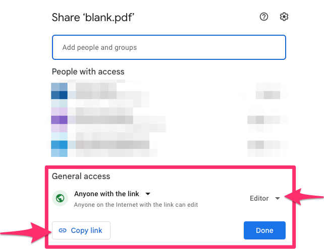
Step 3: Now you have the link, it will look like this:
https://drive.google.com/file/d/<file ID>/view
(file ID will be unique to each file)
Step 4: Now you can paste it into the text box in the Insert hyperlink dialog box.
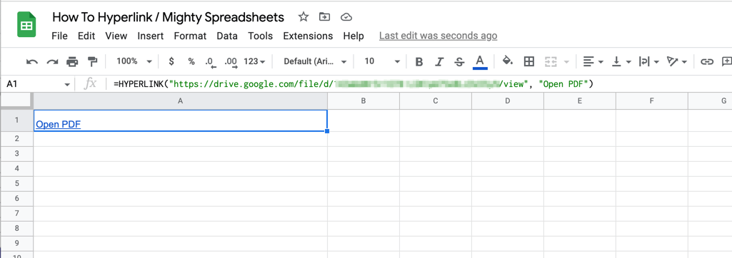
Step 5: When you click on the link it will open the PDF in a new tab
Final Thoughts
Well, now you know how to create, add and edit hyperlinks in Google Sheets.
We covered 4 different ways of creating hyperlinks in your worksheet (which one is your favorite?) and 5 creative ways of using them
I hope this article answered all questions you had about adding links to Google Sheets but if I’ve missed something then please let me know in the comments below!