How to Remove Gridlines in Google Sheets (Ultimate Guide)

This tutorial aims to give you a definitive guide on how to hide, show, and print with or without gridlines in Google Sheets.

It should take you around 5-10 minutes to complete. You may follow along using the spreadsheet available here (just make a copy and you are ready to go).

How to Get Rid of Gridlines In Google Sheets

You can easily get rid of lines in Google Sheets in a few clicks using the Options Menu. These are the steps you need to follow:

Step 1 (Optional): Make a copy and open the exercise spreadsheet in your Google sheets

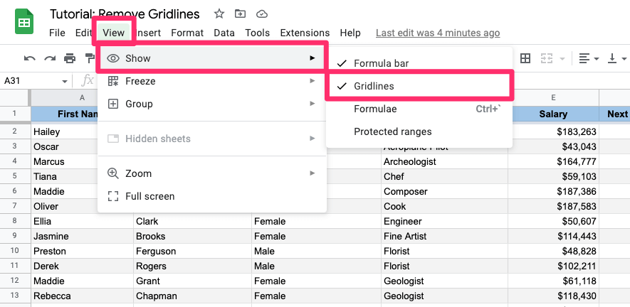
Step 2: In your Options Menu navigate to View > Show and then click on the “Gridlines”

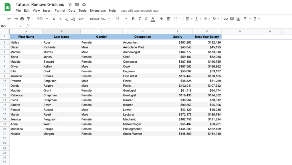
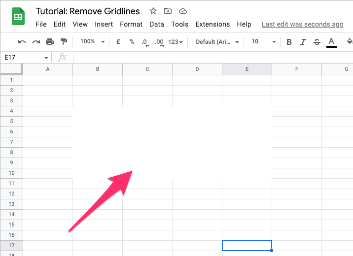
That’s all it takes, your gridlines are gone for good. Simple, right?

Note: Unfortunately, this operation only removes gridlines for your current worksheet. If you want to remove them on all worksheets, you will have to repeat the process multiple times.

How to Show Gridlines In Google Sheets

If you want to have your gridlines back, follow the same process as before. Go to View > Show and click “Gridlines” to revert your worksheet.

The following chapters will provide a more in-depth look at other potential problems you may be facing while working on your document. We will remove gridlines for the print view and hide gridlines only for a specific axis.

Let’s go!

How to Print Without Gridlines in Google Sheets

That’s very often confusing but even though you removed the grid and there are no lines in your worksheet the gridlines are still appearing when you try to print it.

It may be annoying but it’s not hard to hide them in the printing mode either. Here’s what you need to do:

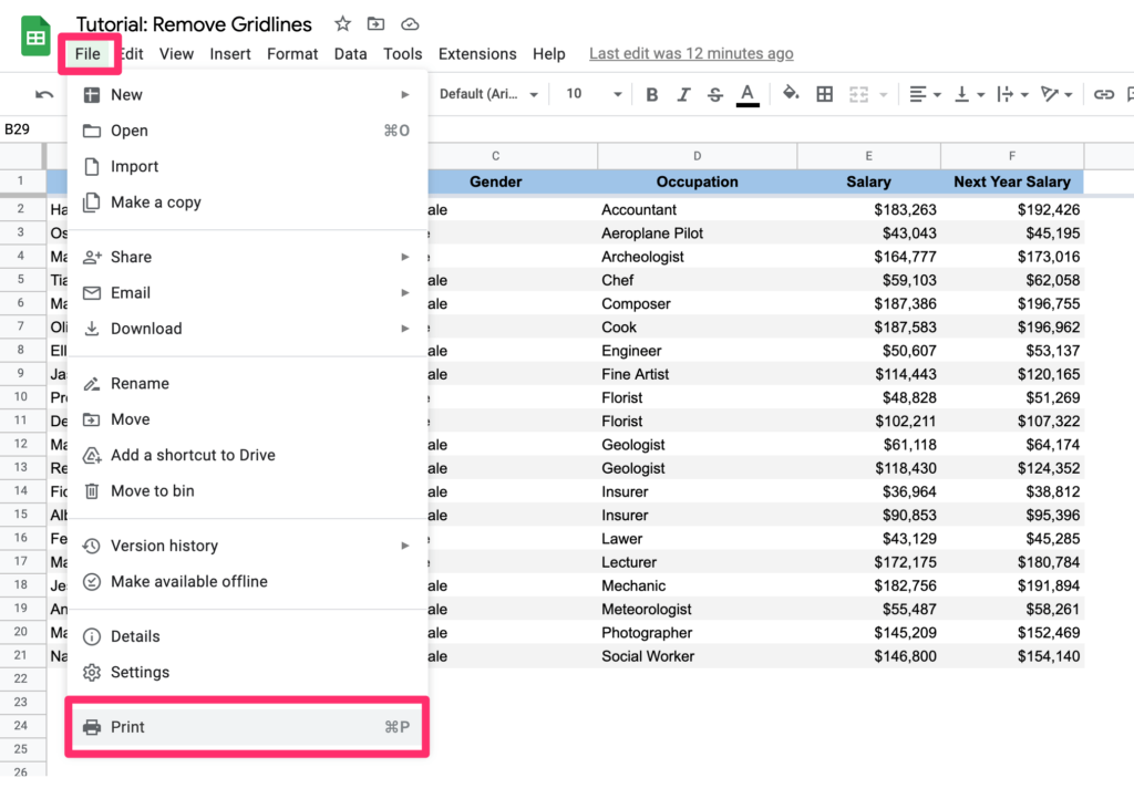
Step 1: In the Options Menu go to File > Print (or just use COMMAND/CTRL + P shortcut)

Step 2: Observe that the gridlines are still visible

Step 3: Find the “Formatting” section in the right-hand side menu and untick the “Show grid lines” checkbox

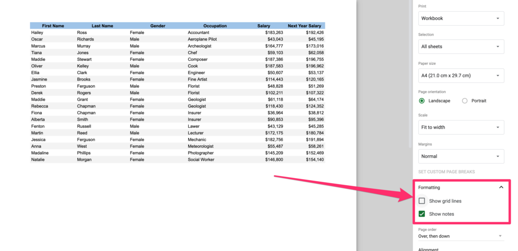
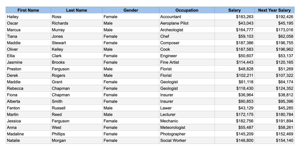
Done, you can now print your worksheet without any additional lines.

How Do I Remove Gridlines From Certain Cells?

If you ever need to only remove cell lines from a limited range of cells you will quickly notice that it’s not possible by default.

However, there’s a workaround that’ll give the appearance of gridlines not being present.

Here’s how to do it:

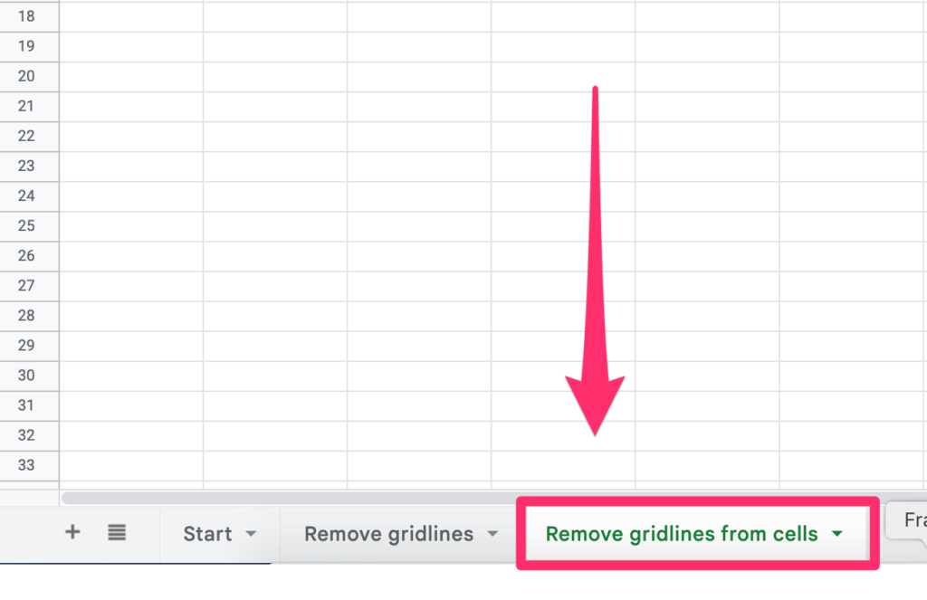
Step 1 (Optional): If you are following along with the exercise sheet, open the “Remove gridlines from cell” sheet

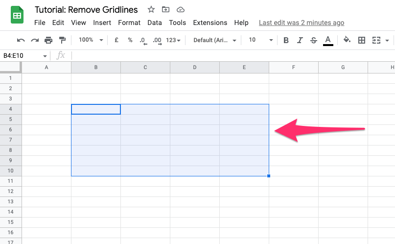
Step 2: Highlight the cells that you want to remove the gridlines from

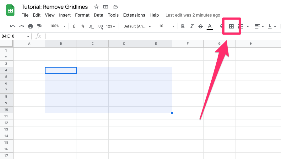
Step 3: Click on the “borders” option from the toolbar menu

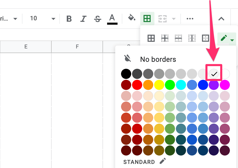
Step 4: Select the border color to be white

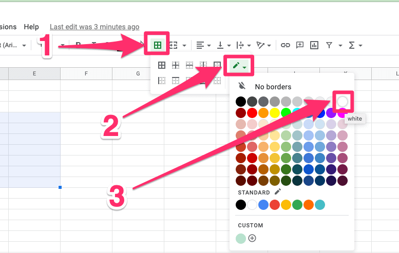
Step 5: Click on the “All borders” button

Done, you just removed gridlines from the selected cells!

How Do I Get Rid of Vertical Gridlines in Google Sheets?

If you want to show only horizontal lines, the process is similar to what we did before. The only difference here is that you need to select “Vertical borders” from the Borders contextual menu instead of “All borders”.

Here’s how it works:

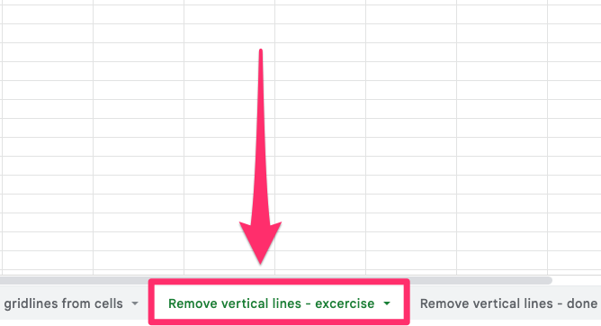
Step 1 (Optional): If you are following along with the exercise sheet, open the “Remove vertical lines – exercise” sheet

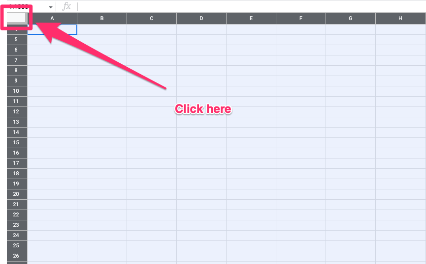
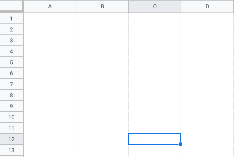
Step 2: To highlight the entire worksheet, click on the small square in the upper left corner.

Step 3: Click on the “Borders” option from the toolbar

Step 4: Select the border color to be white

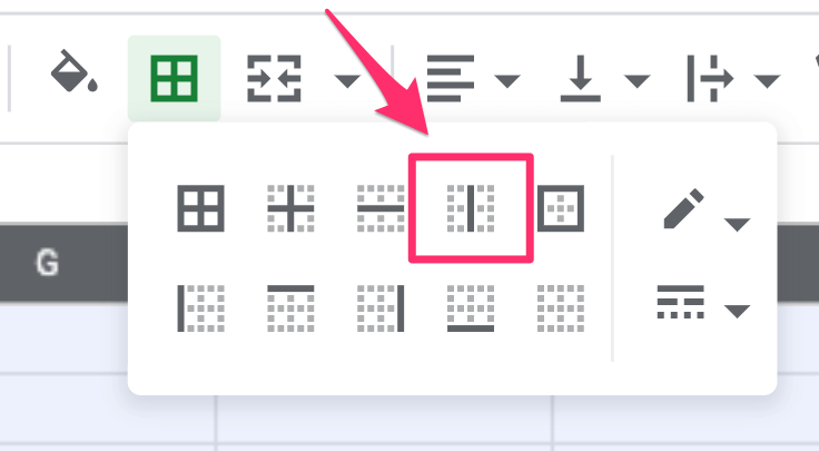
Step 5: Click on the “Vertical borders” button

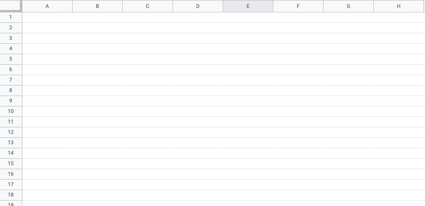
Done, you successfully removed the vertical grid

How Do I Get Rid of Horizontal Gridlines in Google Sheets?

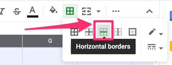
If you want to remove horizontal lines, the process will be quite familiar to you right now. The only difference here is that you need to select “Horizontal borders” from the Borders contextual menu instead of “All borders”.

Here’s how it works:

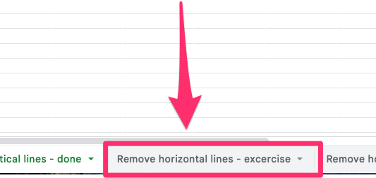
Step 1 (Optional): If you are following along with the exercise sheet, open the “Remove horizontal lines – exercise” worksheet

Step 2: Highlight the whole worksheet

Step 3: Click on the “Borders” option from the contextual menu

Step 4: Select the border color to be white

Step 5: Click on the “Horizontal borders” button

Done, you successfully removed all vertical lines and only horizontal ones are visible!

How to Hide Gridlines in the Google Sheets Mobile app? (iPhone, Ipad, Android)

The process of hiding gridlines in the mobile app is a bit different but still very simple. Here’s what you need to do:

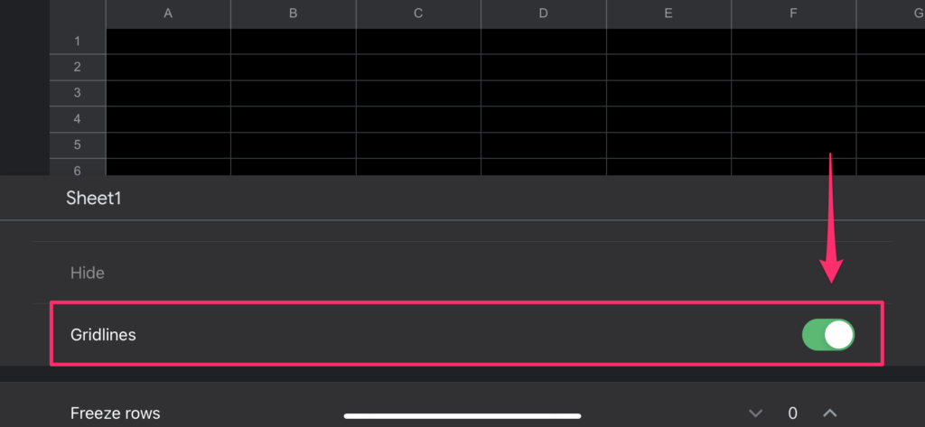
Step 1: Tap on the green arrow icon next to your worksheet name

Step 2: Scroll down to the “Gridlines” toggle and check it off

Some Questions You May Have

What to do if gridlines are missing In google sheets?

If the gridlines are missing in your Google Sheets, that means somebody else turned them off. To turn them back on, go to Options Menu > View > Show and click “Gridlines.”

If this doesn’t help that means that gridlines are present but their color was changed to white. All you need to do is to select the “Borders” icon from the toolbar menu:

Change the color to light gray

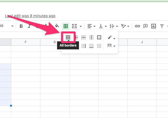
And click on the “All borders” option

My Final Thoughts

Gridlines that appear on a spreadsheet help with alignment and visual clarity but there are many reasons why may like to turn them off.

As we saw today, it’s a very simple process that can be completed in just a few clicks no matter if you want to remove them completely, or partially (i.e. only vertical or horizontal ones) or for printing purposes only.

I hope you found this post helpful. If you have any questions or comments, please leave them below. I would love to hear from you!