If you want to learn how to freeze rows, columns, and panes in Google sheets you are in the right place.
In this tutorial, I will teach you how to:
- keep the top row of google sheets always visible so you can easily see which heading the data is referring to,
- how to make a column stay on the left-hand side when you need to scroll horizontally
- and how to combine both things together at the same time.
The tutorial should take you around 10 minutes to complete. You may follow along using the spreadsheet available here (just make a copy and you are ready to go).
- How to Freeze Rows In Google Sheets
- How To Freeze Columns In Google Sheets
- How To Freeze Multiple Columns In Google Sheets
- Freezing Panes in Google Sheets
- How to adjust frozen rows and columns in google sheets
- How to unfreeze rows in google sheets
- How To Freeze and Unfreeze on Mobile devices? (iPhone, Ipad, Android)
- Some Questions You May Still Have
- My Final Thoughts
How to Freeze Rows In Google Sheets
In this section of the tutorial, we will focus on multiple variations of freezing rows. Here’s what I’m going to cover:
- How to keep a single row on the top of your spreadsheet
- How to freeze multiple rows
Let’s go!
How To Pin a Single Row in Google Sheets
Actually, I like how easy it is to make a row float. And you can do it in two ways:
Using your mouse to freeze a row:
Step 1 (Optional): If you copied the testing sheet you can open the “Freeze single row” tab
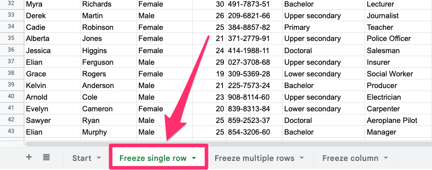
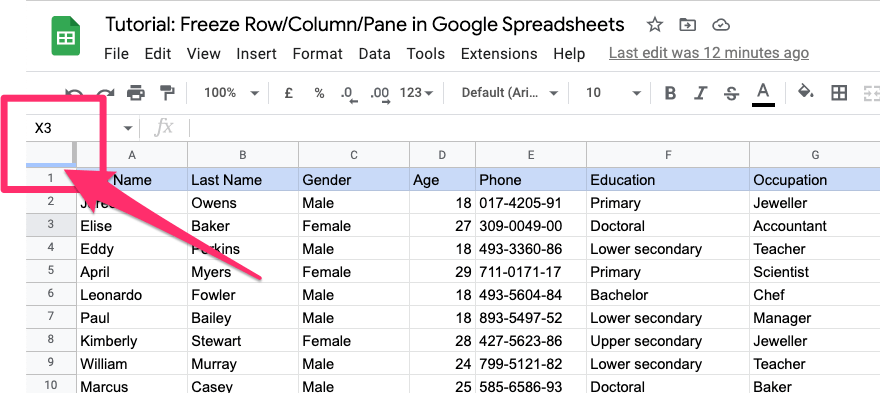
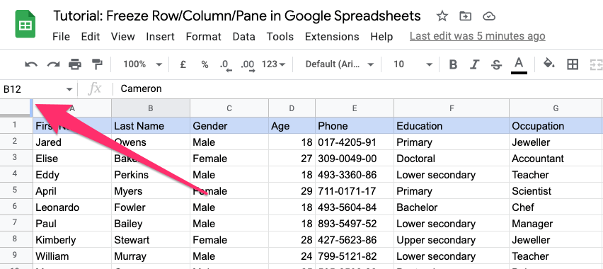
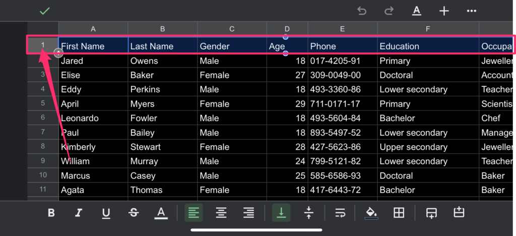
Step 2: Look at the upper-left corner of the current worksheet. You will see a blank gray box with two thick gray lines. Just hover on the bottom line (it should highlight in blue)
Step 3: Click on it and drag the line between rows 1 and 2.
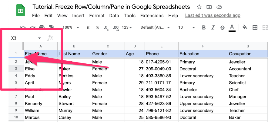
Step 4: You have now made the header row fixed. Just scroll down to see how it sticks.
Using the options menu:
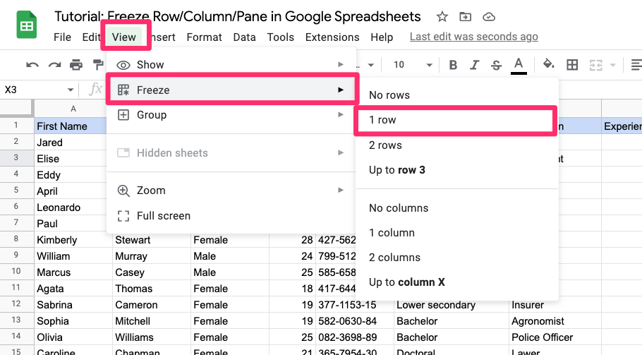
You can also achieve the same effect by using the options menu. All you need to do is navigate to View > Freeze and then click on “1 row”. This will create the exact same output.
How To Freeze Multiple Rows In Google Sheets
Ok, I showed you two ways to have a top row always visible, but what if you want to know how to freeze more than 2 rows in Google Sheets?
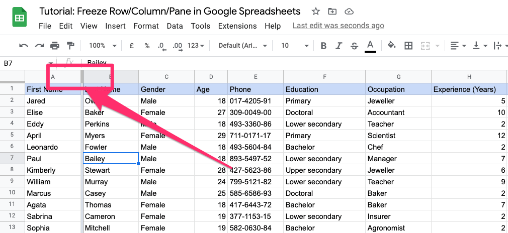
Step 1: If you are following along with the exercise sheet open the “Freeze multiple rows” tab.
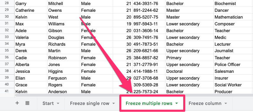
Step 2: Hover your mouse over the lower, thicker line in the blank gray box on the top left corner of your current worksheet.
Step 3: Click on it and drag the line behind the 3rd row
Done! That’s all you need to keep multiple rows on top of your spreadsheet.
Alternatively, you can do the same thing using the Options Menu:
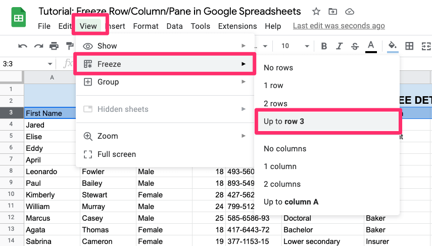
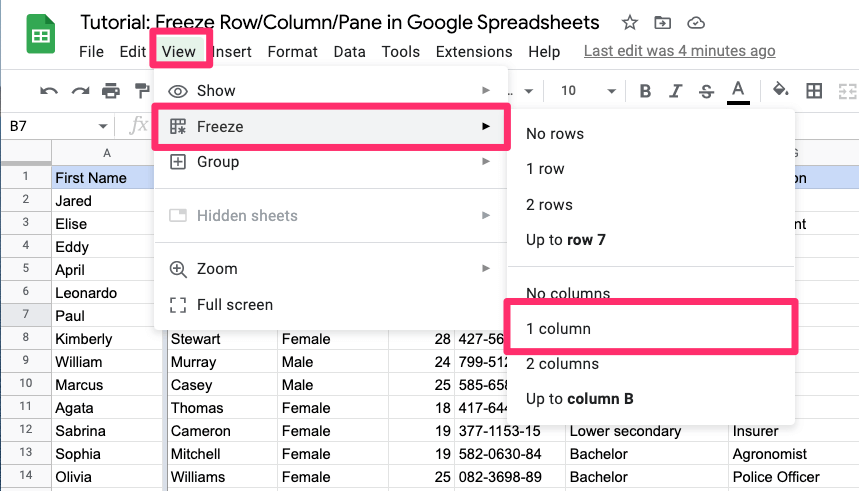
Step 1: Just click on the row that you want to be the last fixed row (in our case it will be row number 3)
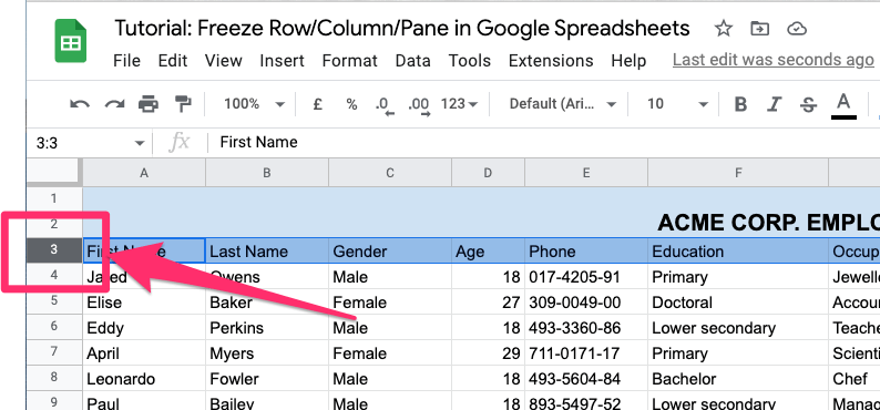
Step 2: Go to View > Freeze and select “Up to row 3”
Things you can’t do with rows
Although it may appear to be a convenient solution, you can’t lock the scroll for the bottom row of your spreadsheets, or any row in the middle of your entries.
How To Freeze Columns In Google Sheets
Well, you already know that. Well kinda. The process is very similar, you are just dragging a different line or clicking another option from the Options Menu:
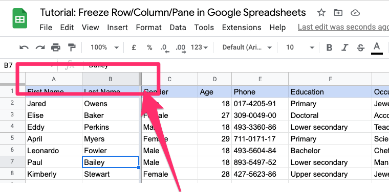
Step 1: Hover your mouse over the thick line that is on the right side of the gray box of your current worksheet
Step 2: Click on it and drag the line behind the 1st column
If you want to do the same from the Options Menu, go to View > Freeze and choose “1 column”
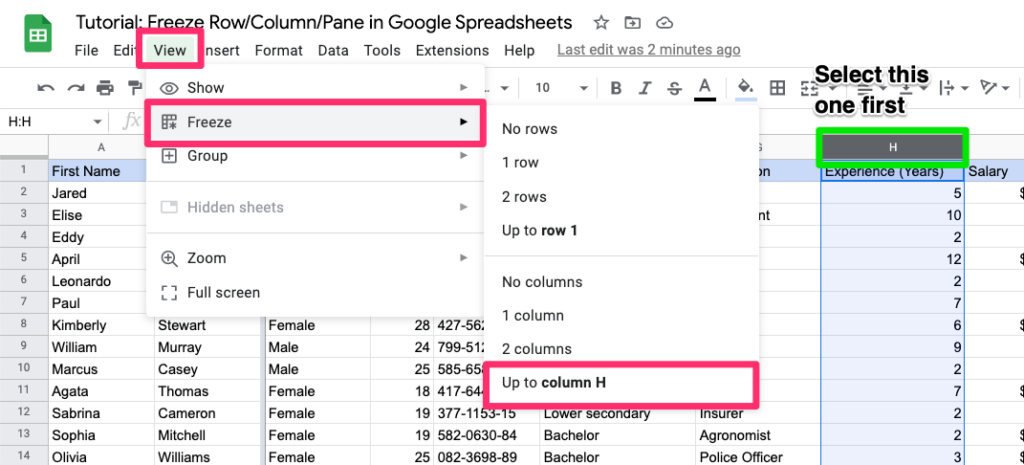
How To Freeze Multiple Columns In Google Sheets
I assume that you already know what to expect here.
Step 1: Hover your mouse over the thick line that is on the right side of the gray box of your current worksheet
Step 2: Click on it and drag the line behind the last column you want to freeze
You can also achieve the same through the Options Menu panel. Click on the last column that you want to be frozen. Then just go to View > Freeze and select “Up to column [letter]”
Freezing Panes in Google Sheets
Just a quick sidenote – you may see the terms “panes” and “columns/rows” used interchangeably.
So to freeze columns and rows at the same time, simply follow the steps I outlined in previous chapters. I bet you shouldn’t have any problems with that but if you do feel free to get in touch.
How to adjust frozen rows and columns in google sheets
Now that you know how to keep your rows and columns in place, it’s time to learn how to change the number of frozen rows and columns.
To do that simply:
Step 1: Hover your mouse over the thick gray line
Step 2: Select it and drag it behind the column or row that needs to be the final sticky one.
Alternatively, if you prefer to do it from the Options menu, just click on the last column/row you want to be frozen (let’s say you want to adjust it to the 5th row), then go to View > Freeze and select “Up to row 5”
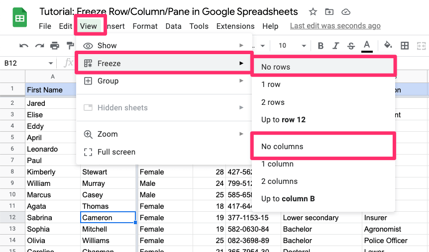
How to unfreeze rows in google sheets
In case you haven’t noticed unfreezing rows is a very similar process to adjusting rows, the only difference is that you set the number of rows to 0
Step 1: Hover your mouse over the thick gray line
Step 2: Click on it and drag it to the very beginning of your worksheet
You can do it from the Options menu too if it’s something that you prefer. Just go to View > Freeze and select “No rows”.
If you are wondering how to unfreeze columns in google sheets then you also have your answer because you need to follow the very same steps in this case.
How To Freeze and Unfreeze on Mobile devices? (iPhone, Ipad, Android)
don’t worry if you’re using Google Sheets on your mobile device – the process is slightly different but still easy to follow.
How to Freeze Rows and Columns in Mobile App (iPhone, Ipad, Android)
Here’s the easiest way to freeze rows and/or columns in the mobile app:
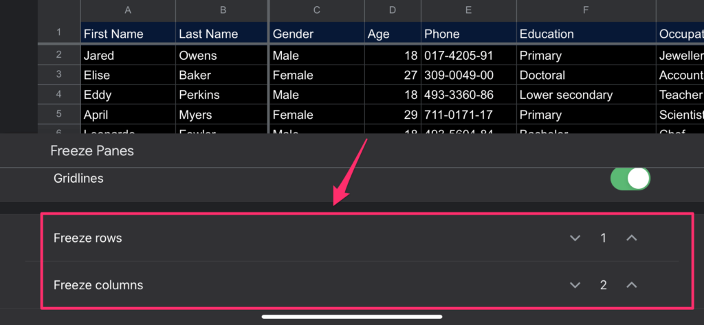
Step 1: Tap on the green arrow icon next to your worksheet name
Step 2: Scroll down to the “Freeze panes” section and just select the value you need from the picker
It’s the easiest and fastest way to do so but it’s not the only way to achieve it
An alternative option to freeze panes in Google Sheets mobile app
Here’s what you need to do if you want to do it in a different way:
Step 1: Open up our worksheet in your Google Sheets App
Step 2: Double-click on the row or column that you want to freeze (if you want to have more rows or columns visible just tap on the last one that needs to be sticky)
Step 3: Scroll right through the contextual menu until you will see the “Freeze row” option.
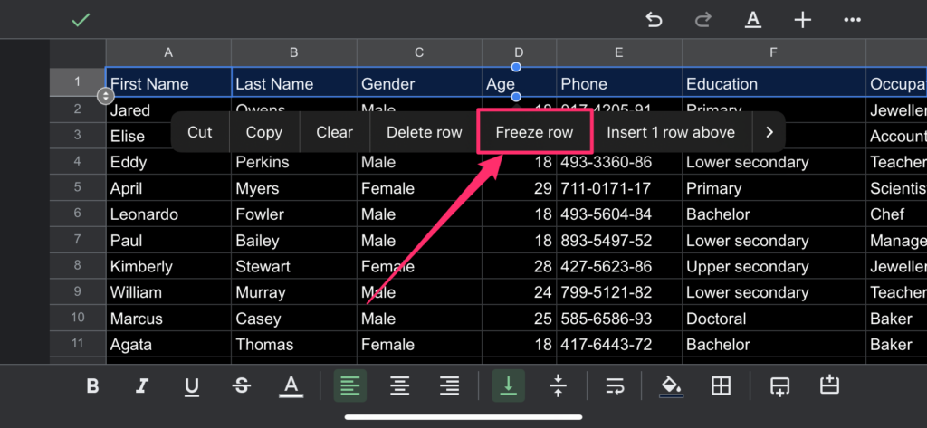
Step 4: Tap on it to confirm. Done, your row or column will not move when you keep scrolling.
How to Unfreeze Rows and Columns in Mobile App
The process of. unfreezing rows and columns in the mobile app is very similar to what we did a second ago to keep it fixed.
Just follow these steps:
Step 1: Double-click on the row or column that you want to unfreeze
Step 2: Scroll right through the contextual menu until you will see the “Unfreeze row” option.
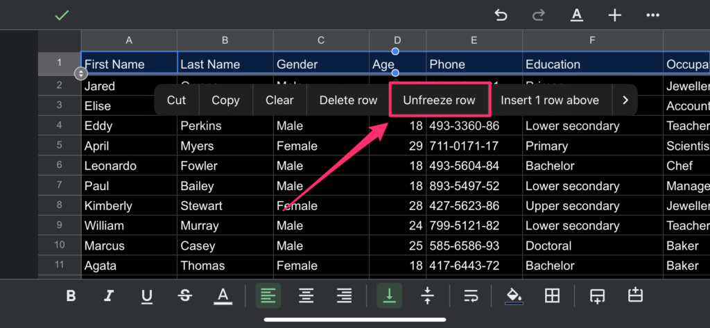
Step 3: Tap on it to confirm.
Some Questions You May Still Have
What is Freeze in Google Sheets?
The term “freeze” is used to describe when a row or column becomes sticky and remains visible even as you scroll down the document.
Can You Freeze a Single Cell?
No, you can’t freeze a single cell in Google Sheets. You can freeze an entire row, multiple rows, a column, a few columns, or a pane at the same time and that’s all.
How many rows can you freeze in Google Sheets?
I was curious about it too and I checked it! Theoretically, you can freeze as many rows as you want, but practically it doesn’t make sense to freeze more rows that fit on your screen.
Google Sheets are smart enough and when you do so you will see a “The current window is too small to display this sheet properly. Consider resizing your browser window or adjusting frozen rows and columns” notification. Which I think is quite useful.
Why would you want to freeze rows in your Google sheet?
Freezing rows or columns is very useful when you are working with large data sets because it allows you to keep an overview of your data while you are scrolling down.
It can also be helpful if there are certain headers or labels that you want to keep visible at all times.
My Final Thoughts
Now you know how to freeze rows and columns in Google Sheets. Frozen rows and columns remain visible when you scroll down the document, which is useful for large data sets or when you want to keep certain headers or labels visible.
You can freeze an entire row, multiple rows, a column, or a few columns at the same time. The process is slightly different on mobile devices but still easy to follow.
If you have any questions or comments, please let me know!