How To Alphabetize in Google Sheets (To Keep List In Order)

If you want to learn how to alphabetize data (or simply stated, put it in ABC order), then you are in the right place.

In this tutorial, I’ll teach you how to organize single columns and multiple columns in alphabetical order in Google Sheets. We’ll also look at two methods for automating this process when your data is updated on a regular basis. Finally, we will do the same things using the Mobile App.

This tutorial should take you around 10-15 minutes to complete. You may follow along by copying the spreadsheet available here

How To Sort Alphabetically in Google Sheets on Desktop (Windows / Mac)

In this section, we will cover the web version of Google Sheets. If you are interested in learning how to do it using a mobile app, just scroll down here.

How To Alphabetize a Column in Google Sheets

It’s quite easy to sort a column alphabetically in Google sheets. You can do it in 3 simple steps:

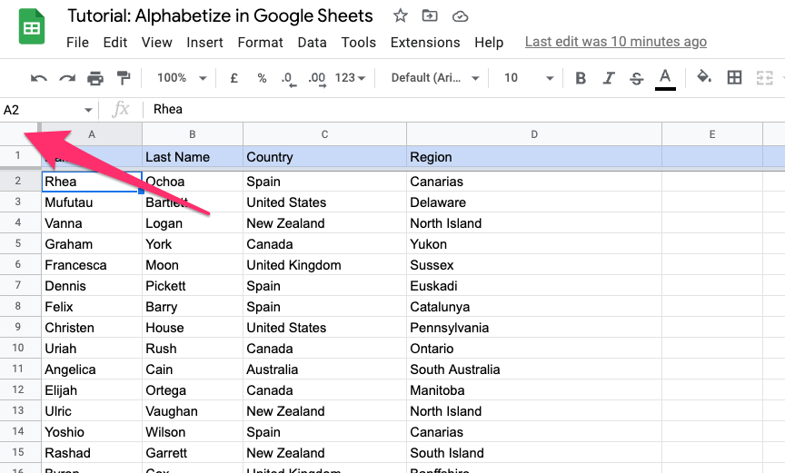
Step 1: Select all table entries (including headers)

The quickest way to select all columns and rows is to click on the blank rectangle that you can see above row number 1 and to the left of Column A.

PRO TIP: If the table is not the only data on your spreadsheet, you can easily select only the rows you want by typing your range in the “name box”.

In this example, we need to enter:

A1:D56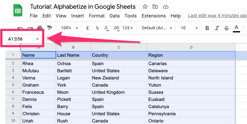

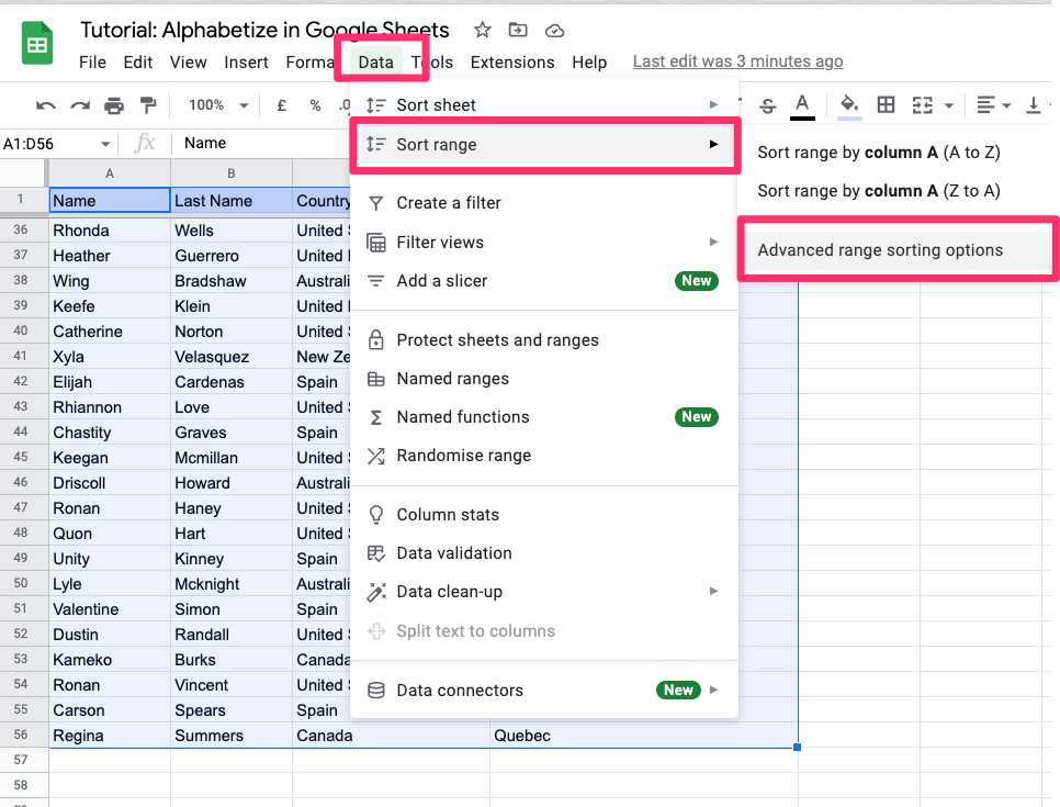
Step 2: Go to Data > Sort range > Advanced range sorting option

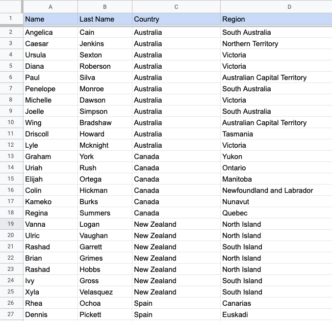
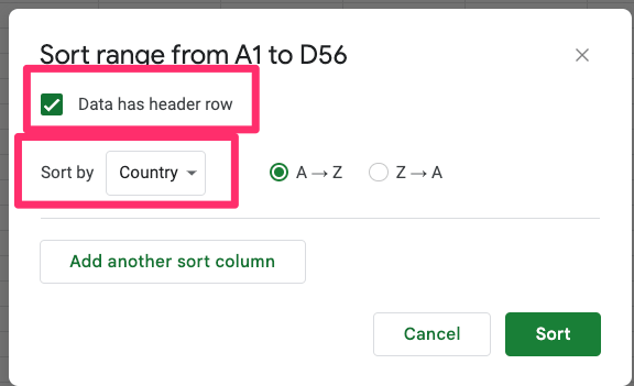
Step 3: Check the “Data has header row” checkbox, select “Country” from the drop-down menu in the “Sort By” area, and click on the “Sort” button.

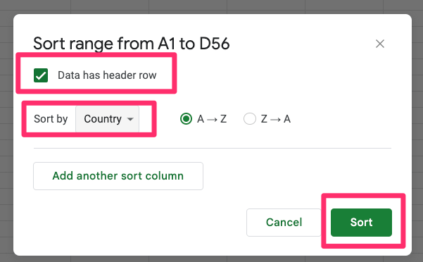
Done, your list is now sorted alphabetically by the “Country”. You can do it with every column that we have in our spreadsheet i.e. you can sort by last name or first name too.

How to Alphabetize By More Than One Column

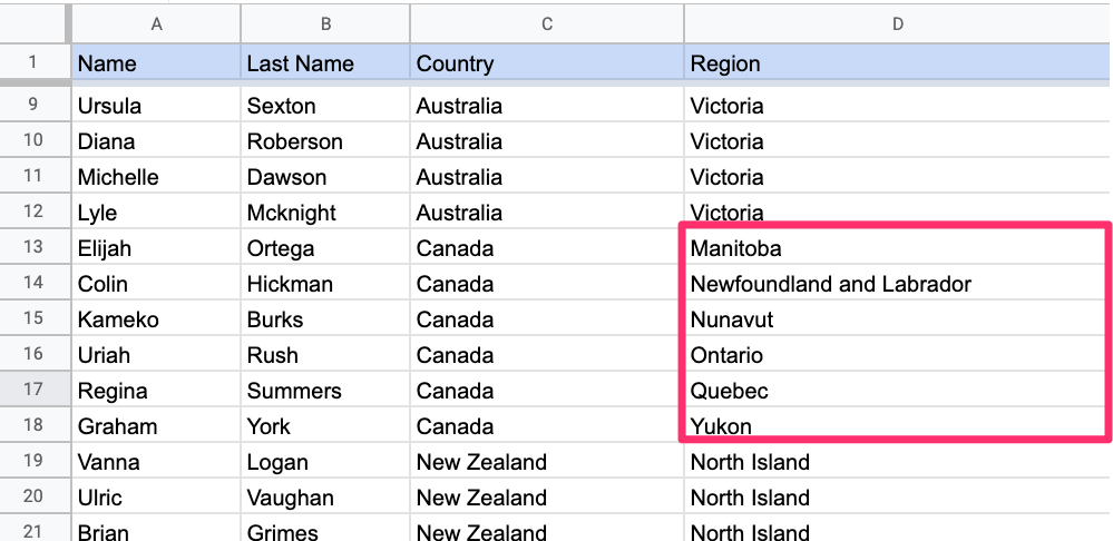
This section will show you how to organize multiple columns in alphabetical order. For example, if you want to sort your list by “Country” first and then by “Region”.

Step 1: Make sure all cells you want to sort are highlighted, then navigate to Data > Sort range > Advanced range sorting option again

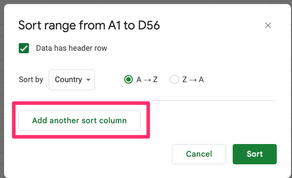
Step 2: Check the “Data has header row” box and pick “Country” for the “Sort By” drop-down list.

Step 3: Click on “Add another sort column”

Step 4: In the “then by” area pick “Region” and click on the “Sort” button

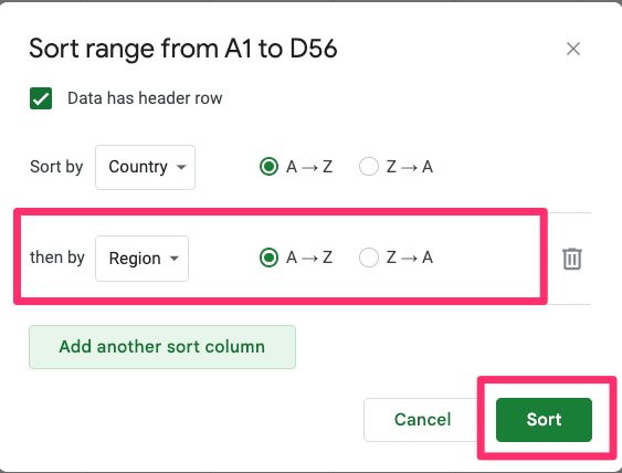
Now you will see that the entries are sorted by two columns now. You can do the same step with as many columns as you want.

How To Automatically Alphabetize In Google Sheets

We’ve got our data sorted, but what if you want to change it in the future? Well, you have two options:

• Option 1: You may repeat the steps you followed in the previous chapter each time your data is updated.
• Option 2: you can use the SORT function that will do it for you
• Option 3: you can create a custom script that will sort the table for you each time you make an edit

Since you already know what to do to cover the first option let’s focus on the second and third ones.

Use SORT function

Using the SORT function is easy and won’t take much time. Let’s see how to sort automatically by alphabetical order with this method:

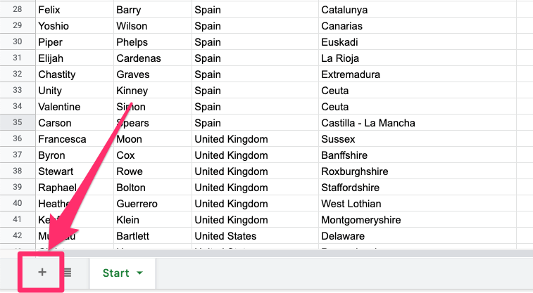
Step 1: Add a new empty sheet to your document

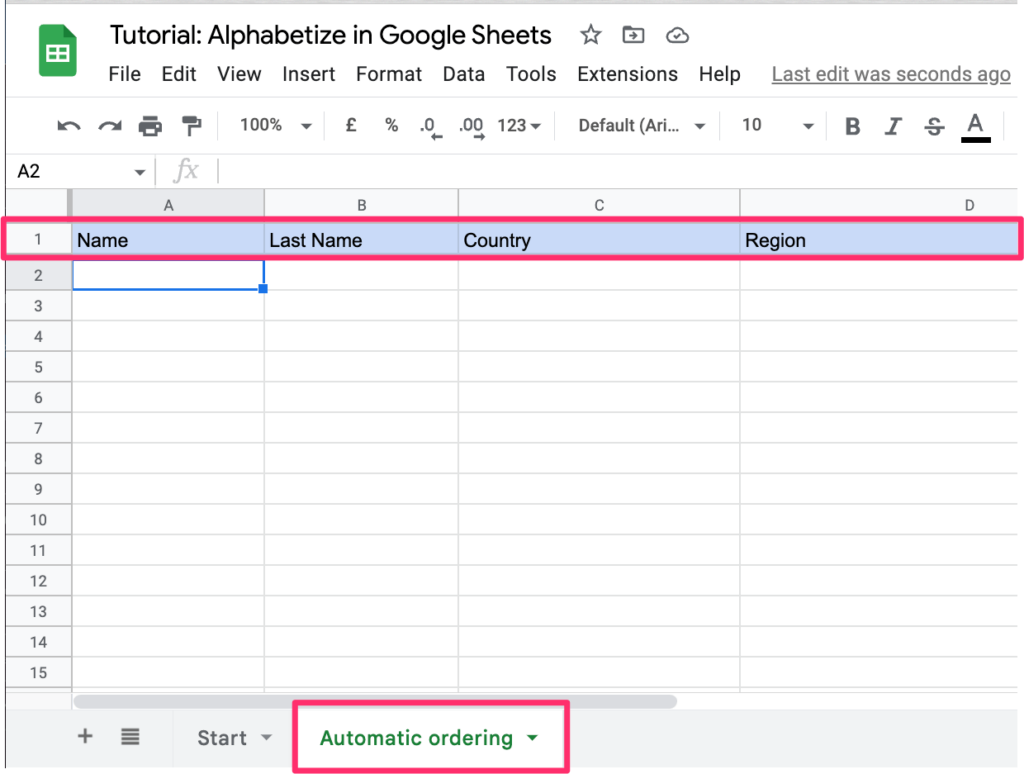
Step 2: Name it however you want (I named it “automatic ordering”). Copy the header rows from the previous document so it looks like so:

Step 3: Click on the A2 cell and paste this function (I will explain the markup at the end of the chapter):

=SORT({Start!A2:D}, 3,1,4,1)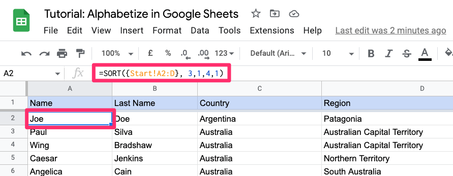

Let’s break this markup a bit so you can understand what you are copy-pasting. This is the syntax for the SORT function:

SORT(range, sort_column, is_ascending, [sort_column2, is_ascending2, ...])

• range – The data to be sorted. In our case we are referring to a sheet called “Start” and it’s range from A2 to D
• sort_column – The index of the column in the range. We put “3” as we are sorting by Country first (it’s 3rd from left)
• is_ascending – TRUE (1) or FALSE (0) indicating whether to sort sort_column in ascending order. We set it to true as we want to have the data sorted in a to z order
• sort_column2 [ OPTIONAL ] – Additional columns and sort order flags beyond the first, in order of precedence. We put the value of “4” because the next column we want to sort is “Region” (4th from left)
• is_ascending2 [ OPTIONAL ] We set it to true as we want to have the data sorted in a to z order too

Step 4: Go back to the “Start” sheet and add a new entry at the end of your document:

Joe, Doe, Argentina, Patagonia

like so:

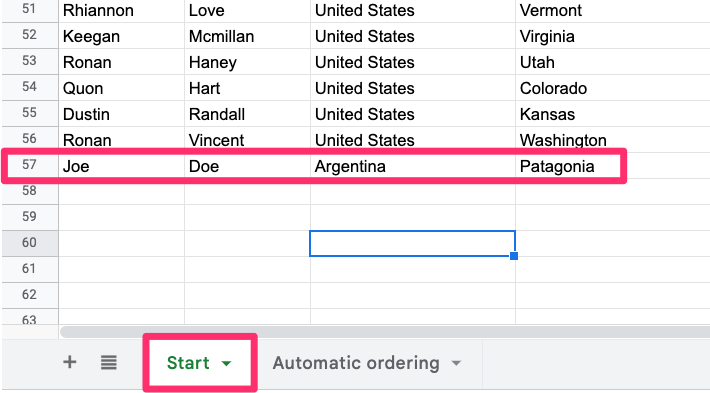
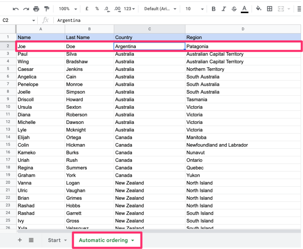
Step 5: Go back to your “Automatic ordering” sheet and see that the result was automatically sorted for you:

Note: The only downside of this approach is that it creates a duplicated set of entries, but very often it is not a problem.

If it’s a problem for you though, then you can write a custom script that will sort your table automatically each time a new entry is added. I will cover it in the next section.

Create custom App Script

I saved this one for the end. I’m well aware that not everyone is tech-savvy and that not everyone needs to know JavaScript. However, if you wish to have a go at it, here’s what you’ll need:

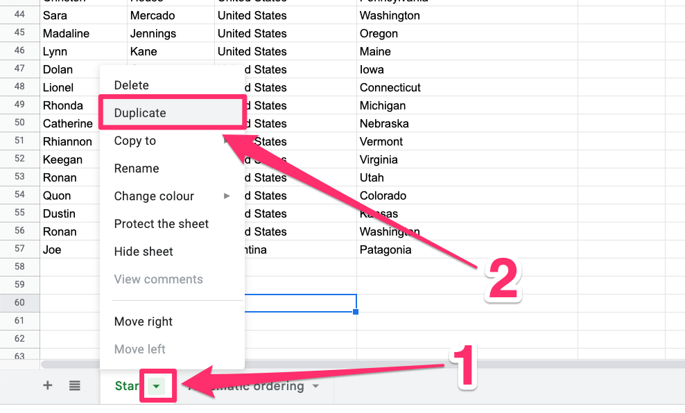
Step 1: Duplicate the “Start” sheet and name it “withAppsScript”

Step 2: Go to Extensions > Apps script.

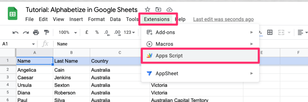
Once you click on it the new project will be opened in a new tab.

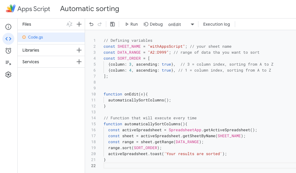
Step 3: Copy and paste the code below.

I left some comments in the code so you can understand it better and update the values if you want to use it on your other projects:

// Defining variables
const SHEET_NAME = "withAppsScript"; // your sheet name
const DATA_RANGE = "A2:D999"; // range of data tha you want to sort
const SORT_ORDER = [
  {column: 3, ascending: true},  // 3 = column index, sorting from A to Z
  {column: 4, ascending: true}, // 1 = column index, sorting from A to Z
];

function onEdit(e){
  automaticallySortColumns();
}

// Function that will execute every time
function automaticallySortColumns(){
  const activeSpreadsheet = SpreadsheetApp.getActiveSpreadsheet();
  const sheet = activeSpreadsheet.getSheetByName(SHEET_NAME);
  const range = sheet.getRange(DATA_RANGE);
  
  range.sort(SORT_ORDER);
  activeSpreadsheet.toast('Your results are sorted');
}

It should look like this:

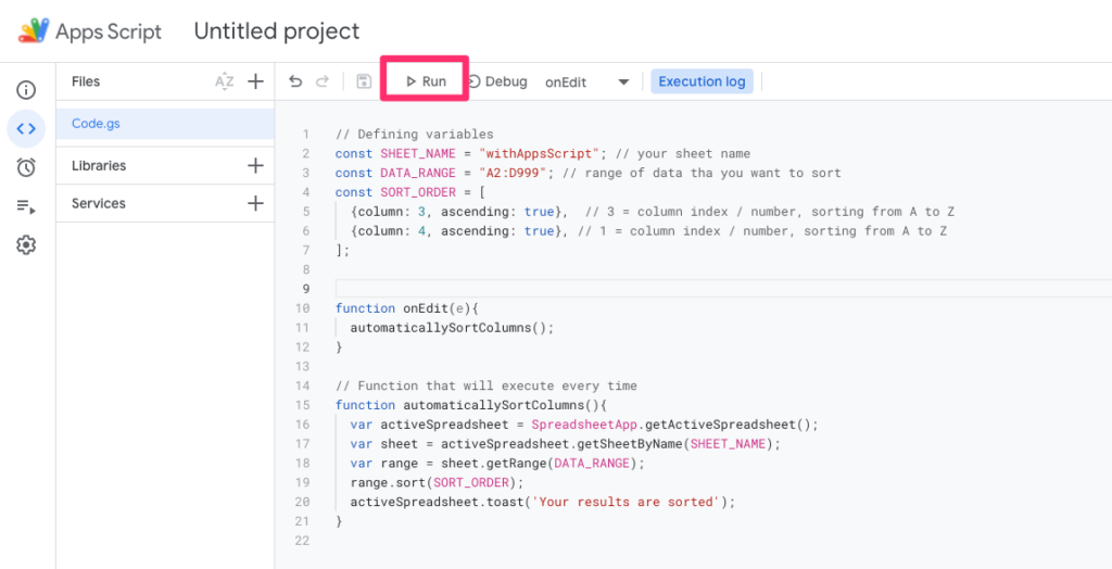
Now, just click on the “Run” button and go back to your sheet:

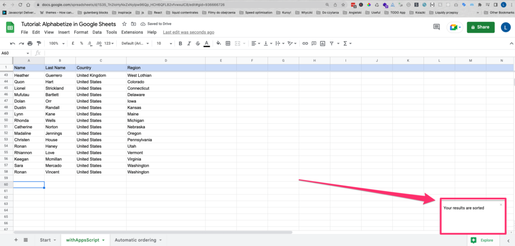
Step 4: Add a new entry, wait for it to be sorted, and look for a notification popup:

Note: This tutorial is designed to help you sort your results in an alphabetical way and it isn’t intended to teach you how to code for Apps Script. As a result, the functionality is quite basic and I’d like to keep it this way.

However, if you want to make the code even more robust you can experiment with running the function only when the “Country” or “Region” cell is updated or even with running the script every hour using triggers

I hope you’re enjoying it so far. In The next section, we’ll be using your phone instead of the web/desktop version. Stay with me.

How To Sort in Alphabetical Order In Google Sheets In Mobile App

When you use the mobile app, certain features differ from the desktop version. Below you will find a helpful guide to sorting a to z in the mobile app:

Note: I use dark mode on my mobile app, if you like what you see then read more about enabling dark mode for desktop and app.

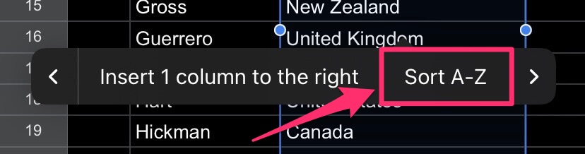
Step 1: Double tap on the column name (in our case on the letter “C”) you would like to sort and the contextual menu will open

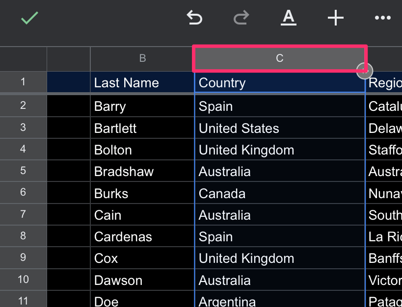
Step 2: Scroll until you see the “Sort A to Z” option and tap it.

Done, your column is now ordered in alphabetical order.

How To Sort Multiple Columns In Google Sheets In Mobile App

There is currently no contextual menu that allows you to arrange many columns, but you may still utilize the SORT function to do so.

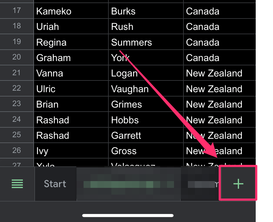
Step 1: Create a new sheet by clicking on the plus (“+”) icon in the bottom right corner.

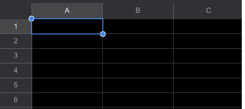
Step 2: Double-tap on the first column (A1) of your new sheet in order to edit the cell’s content.

Step 3: Write the SORT function:

=SORT({Start!A2:D}, 3,1,4,1)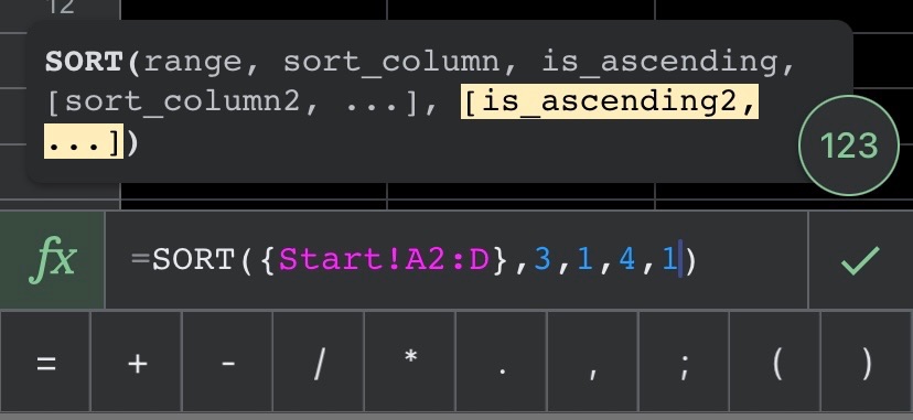

and click on the “Tick” icon to confirm your function.

Step 4: Enjoy! That’s all you need (To make headings rows, you may simply add a new row before the entries.)

Note: If you jumped straight to this section please scroll up for an explanation of the SORT function’s syntax if you want to know what arguments it takes.

Some Questions You May Still Have

My Final Thoughts

The article explains how to sort data in alphabetical order in both the Google Sheets desktop and mobile apps.

In the desktop app, you can do it using the Sort Range option, using the SORT function, or by adding a custom script in Apps Scripts

In the mobile app, you can double-tap on a column name to open a contextual menu that includes the “Sort A to Z” option.

If you have any questions or suggestions, please let me know in the comments below.

Thank you for reading!