How to Make a Data Table in Google Sheets (Like In Excel!)

If you’re used to Excel, new to Google Sheets, or have never created a table before, the task may seem daunting. However, don’t worry! In this article, I will show you how to insert a table into google sheets in just a few simple steps.

You will learn the basics of converting data into a table format, as well as some advanced topics on how to extend your table with more options. Let’s get started!

PS. The tutorial will take approximately 5-15 minutes to complete.

5 Things You Need To Know About Google Sheets Table Formatting

This section consists of 5 formatting tips for making a table in Google Sheets. We will start with raw data and make it neater while we go through all the points. This is what we are going to cover:

1. Creating headings and alternating colors
2. Make column headings sticky
3. Aligning columns
4. Formatting data
5. Naming your table

Note: If you want to follow along with the tutorial, here’s a link to the raw data I’ll be using (created with Random Data Generator). Simply open it, create a copy and join me in the journey (this step is completely optional though).

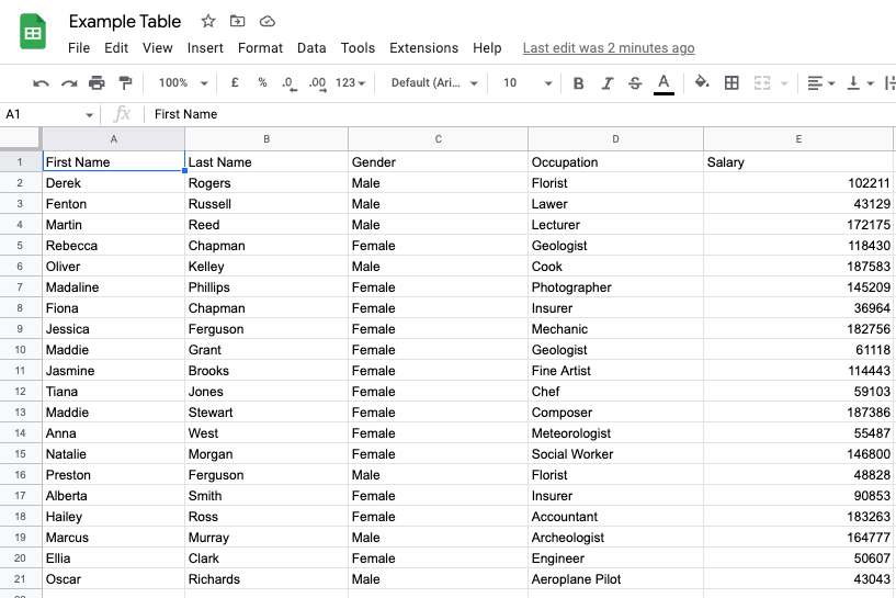
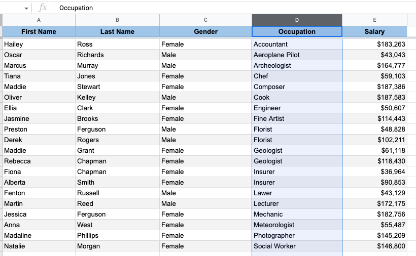
After copying the file this is what you should be seeing:

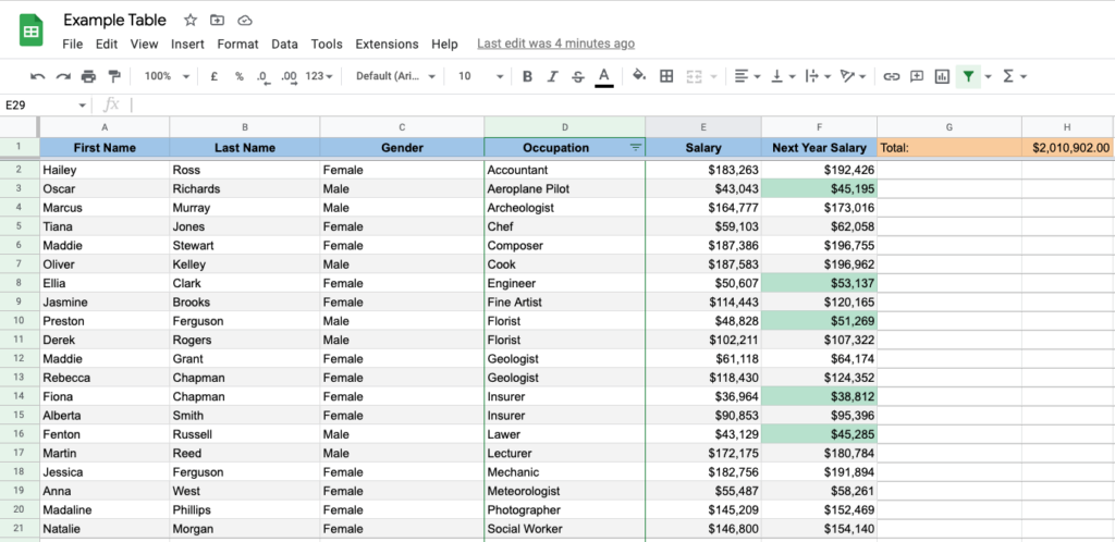
And this is the final result we want to achieve:

Let’s jump straight to the first task.

#1: Creating Headings and Alternating Rows:

Let’s add color to the background of the heading so it stands out, and then we’ll alternate odd/even cells to make them more visually appealing.

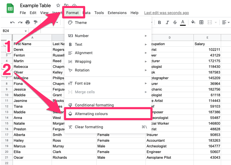
Go to Format > Alternating colors:

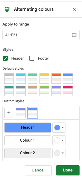
Now pick your desired theme (you can use a predefined one or customize it) and click on “Done”.

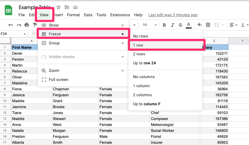
#2: Make Column Headings sticky

When you create a table in google sheets with many entries you may want to make the column sticky so you have a point of reference when you scroll down.

Just go to View > Freeze and select “1 row”:

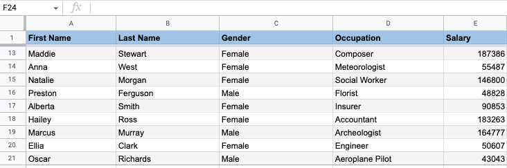
When you scroll down a tiny bit, it will appear like this:

#3: Aligning your data

These are the best practices for aligning the data:

• The text should be always left aligned
• All standardized entries (i.e. IDs) and column headings should be center aligned
• Numbers and dates should be right-aligned

It’s quite easy to align your content. Just go to Format > Alignment and pick the one you need:

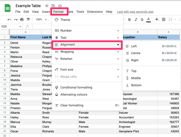
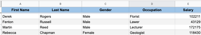
For the tutorial purpose let’s align the table headings to the center (the rest of the values is correctly aligned by default):

PS. There are some shortcuts for aligning the values:

• Press Command + Shift + L for aligning left
• Press Command + Shift + E for aligning into the center
• Press Command + Shift + R for aligning right

#4: Formatting table data

Now let’s use the correct format for the values we’re using.

A salary is simply a number, but it should be represented in monetary units.

It shouldn’t include any decimal places (as opposed to product prices, for example).

In various cases, you may also need to switch to another currency. I will cover this as well.

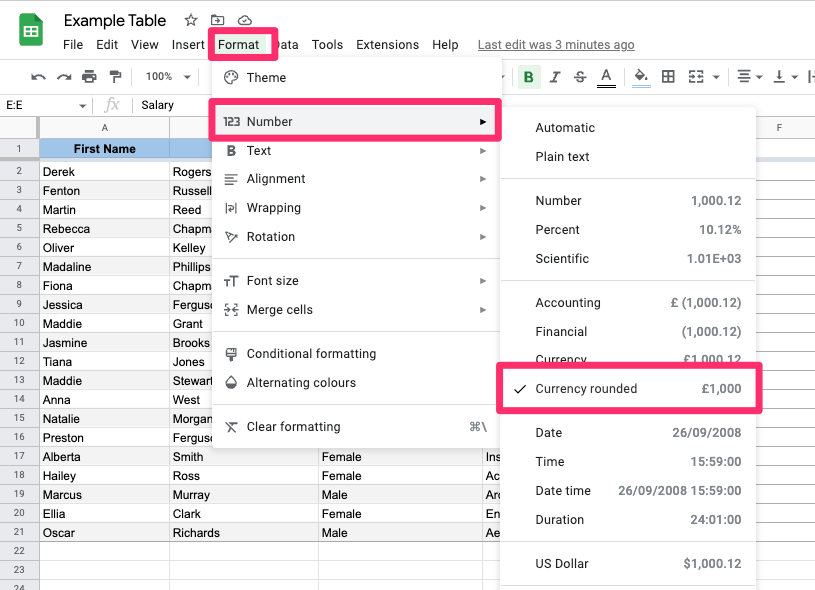
Step 1: Add a currency to your values

Highlight your data (in our case “Salary”) then navigate to Format > Number > Currency rounded to get the value without decimals:

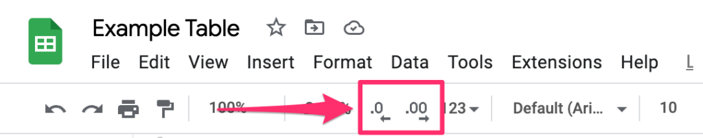
If for some reason you’d like to use the decimals, you can add them from the toolbar menu:

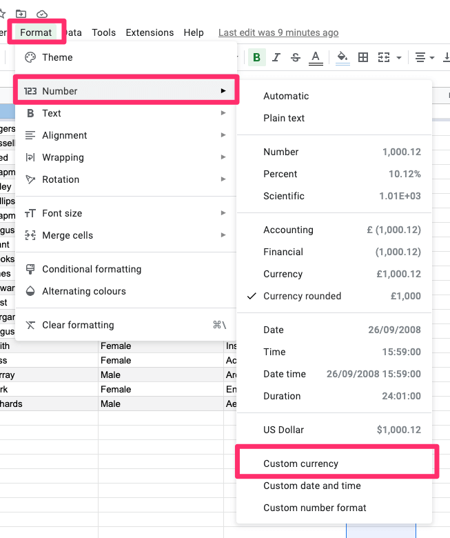
Step 2: Change the currency

Go to Format > Number > Custom currency:

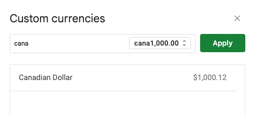
and use the search bar to find the currency you are interested in. Click “Apply” and that’s all.

#5: Naming your table

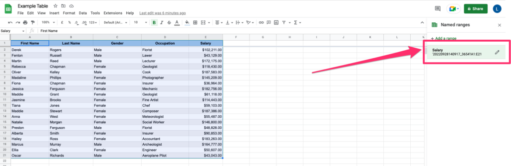
You can make your work with tables in Google Sheets more efficient by naming the table. This creates a named range that allows you to reference your google sheets table later in another spreadsheet just by using its name.

Creating a named range is quite simple:

Step 1: Select all the cells that you want to name (in our case the whole table).

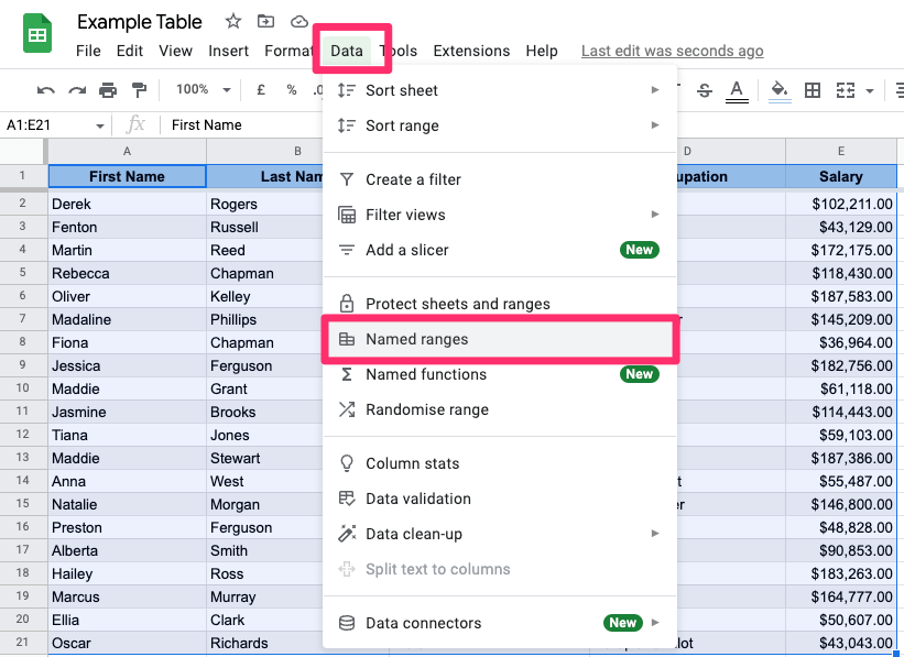
Step2: Click on Data > Named ranges.  

Step 3: Type the range name that you want.

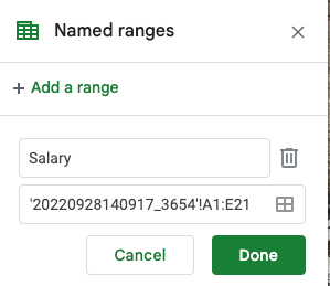
Click Done.

A few tips on naming a range:

• The range can contain only letters, numbers, and/or underscores (that means no spaces!)
• The range can’t start with a number or the words ‘true’ or ‘false’.
• Must be 1–250 characters.

Extending Our Google Sheets Table With Extra Features

In this section, we will go over 4 advanced formatting tips for making tables in Google Sheets more efficient. We will also add some great features to automate some simple processes. Here’s what we are going to cover:

1. Sorting google sheets table
2. Adding total row
3. Filtering google sheets table
4. Automatic calculations
5. Conditional formatting

#1: Sorting Google Sheets Table

We’ll sort two columns at a time for the sake of training; this may come in handy in a variety of situations. We’ll start with the “Occupation” column, which will be alphabetized, and then work our way up to the “Salary” column which will be sorted in ascending order (from lowest to greatest value).

Step 1: Highlight the whole table (you can click on the range we created before)

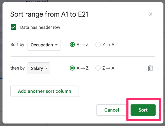
Step 2: Click Data > Sort range > Advanced sorting options

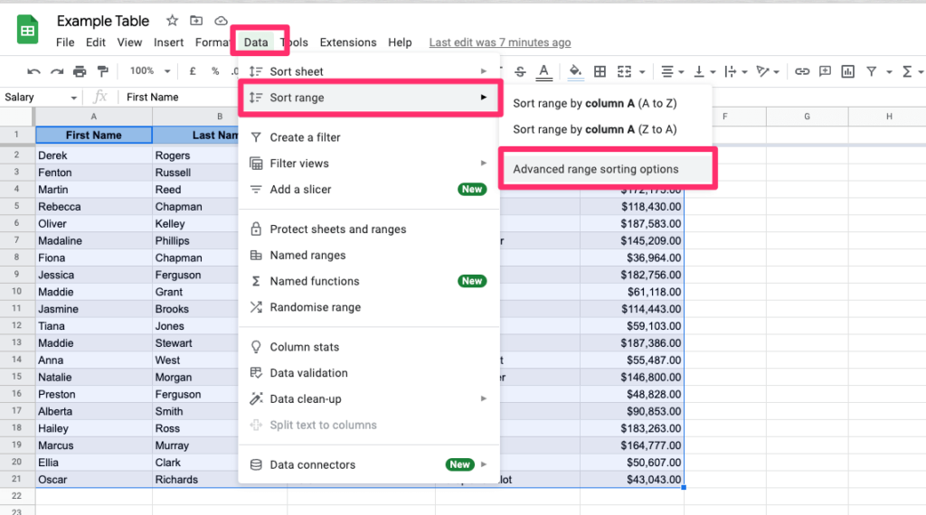
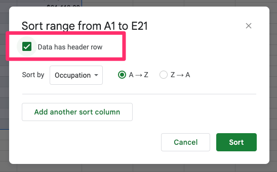
Step 3: Make sure to check “Data has header row” as we don’t want our titles to be sorted

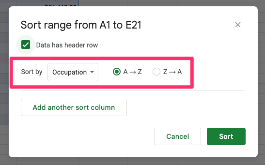
Step 4: Set “Sort by” to “Occupation” and A>Z order

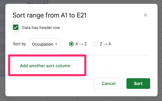
Step 5: Click on the “Add another sort column” button

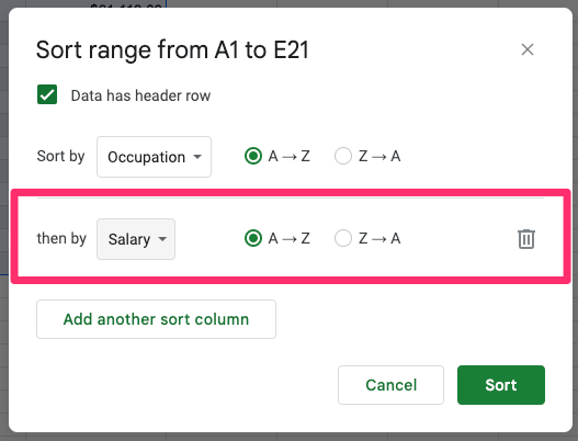
Step 6: Set “Sort by” to “Salary” and A>Z order

Step 7: Click the sort button

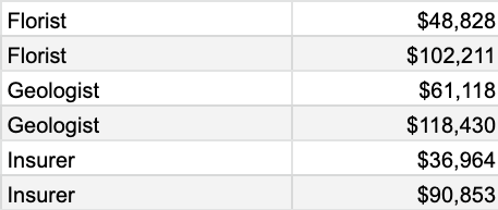
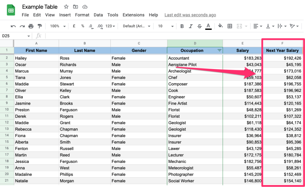
You will see that all the roles are alphabetically sorted and then they are sorted from the lowest value.

#2: Adding a total row

In this section of the tutorial we will cover two things:

• We will sum up all the company’s spending
• Then, we will apply a filter to see how much money each department costs.

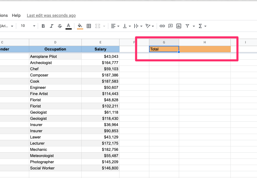
Step 1: In the first row apply an orange background to two cells (“G” and “H” as we will need the “F” column at a later stage). Put “Total” in the first one.

Step 2: In the second cell we will add all the salaries together.

You’re probably thinking of using a SUM function. It appears to be a good idea, but there is one catch. It will just sum up all the values from the cells even if they are hidden.

So if you want the value to adjust when you apply filters to the table, you should use the SUBTOTAL function instead.

Here’s more information about the SUBTOTAL function from the official docs, it will explain why we used “9” as a first argument. (“9” stands for a SUM in SUBTOTAL aggregation function).

Add this to the cell:

=SUBTOTAL(9,E3:E21)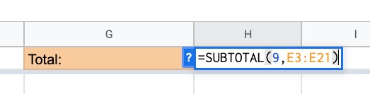

And click Enter

You will see that it appears as a raw number. We need to apply a currency format as we did previously so it looks like that:

Alright, we have the total value that is paid to all employees as a salary. Let’s add some filters now.

#3: Filtering Google Sheets Table

Now let the fun begin. Let’s add some filtering options so for example we can see how much we are paying to the Florists.

Step 1: Highlight the “Occupation” table column

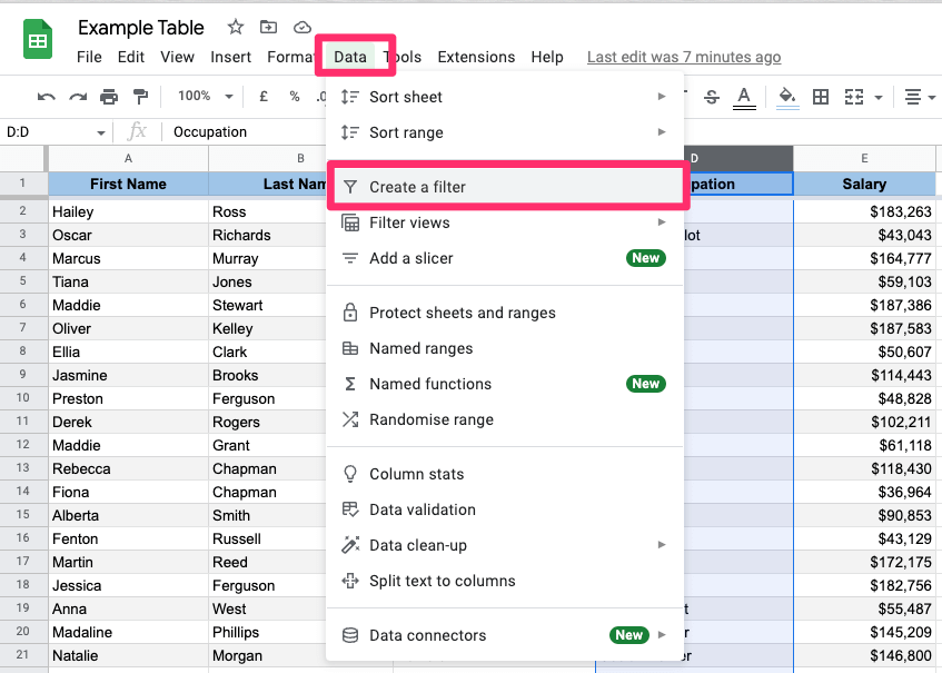
Step 2: Click on Data > Create a filter

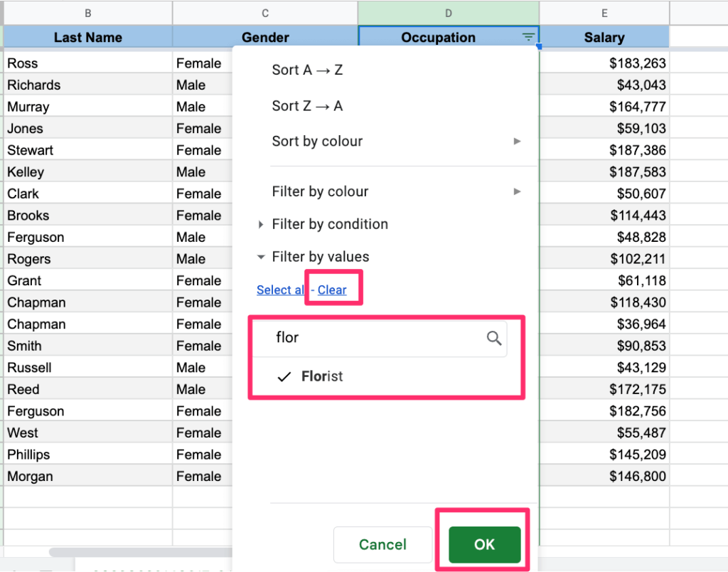
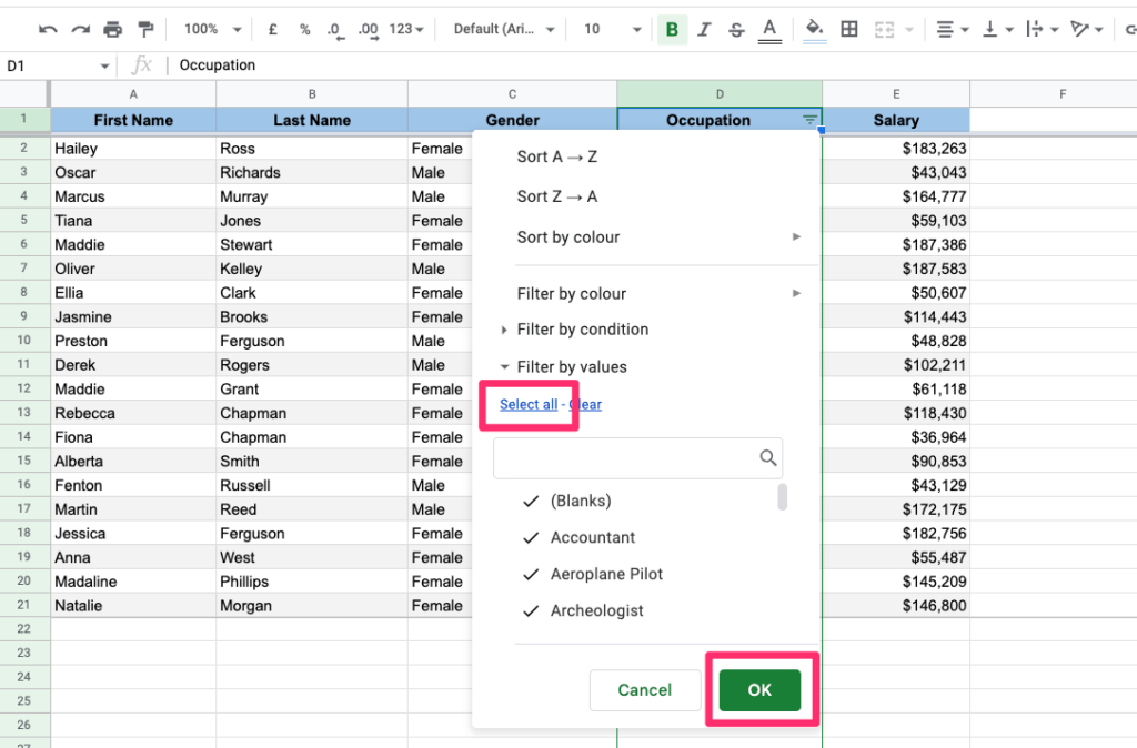
Step 3: Click on the filter icon

Step 4: Clear all selections and type “Florist” in the search bar, then click the OK button.

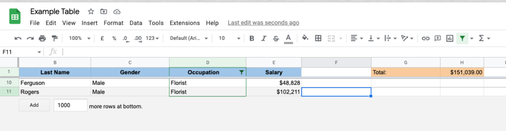
You will see that the table shows only 2 entries and the Total amount has changed as well.

That was pretty easy. Let’s jump to the next step then:

#4: Automatic calculations

Let’s assume that every employee gets a 5% rise each year. Obviously, you wouldn’t like to calculate it manually so let’s just use a simple function that will calculate it for us:

Step 1: Let’s unfilter the data first and show all available entries.

Just click on the filter icon again, click on the “Select All” option and confirm with the OK button:

Step 2: In the “F” column add a new heading which will be “Next Year Salary”

Step 3: Let’s calculate the salary after a pay rise for the first entry.

This is just simple math but you can do more advanced calculations if you want to. Just apply the below to the first entry and click Enter:

=(E2 + E2 * 0.05)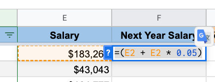

You will see that the amount was automatically calculated for you.

Step 4: Apply the same logic to all other entries

Click on the cell with value and look for a small blue square in the bottom right corner.

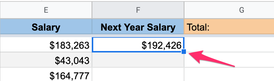
Click on it twice so the values can be populated for all other entries:

All done, you know how much each employee will earn in the next year.

#5: Conditional formatting

As our final step let’s apply some conditional formatting to the table.

If a company wants to pay their employees a minimum salary of $55,000 next year, how can they easily identify who those people are?

Step 1: Highlight the “F” column

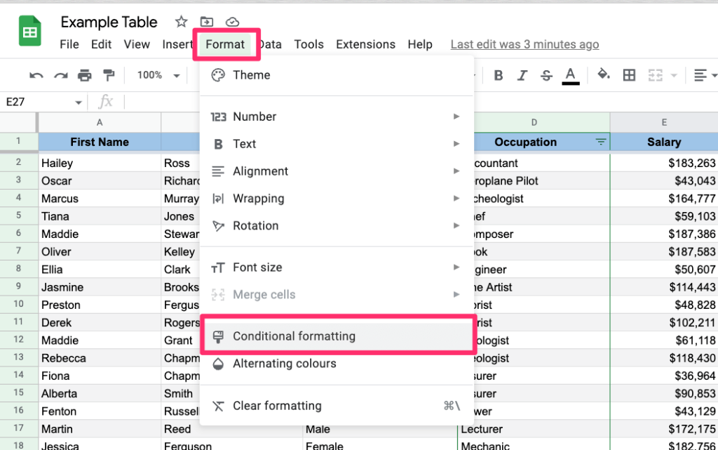
Step 2: Go to Format > Conditional Formatting

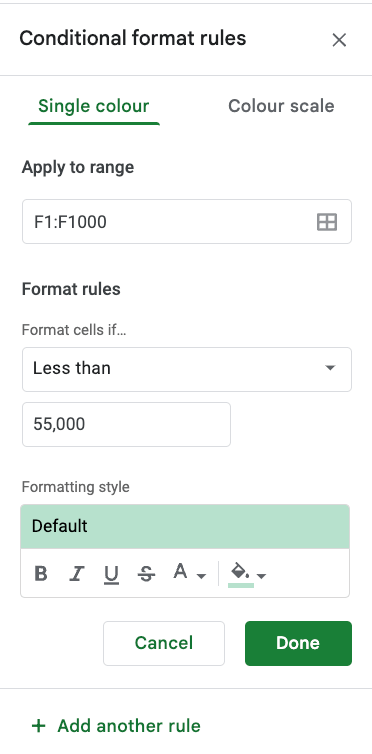
Step 3: Set the Conditional Format Rule

Pick “Less than” and then enter the “55,000” value. You can leave the default formatting style or play with it if you wish

Boom! You can now see who among your staff is due for a substantial raise next year.

Your table should look like this:

Some Questions You May Have

Final thoughts on Making Table in Google Sheets

There you have it. You created a Google Sheet table that looks like the one you can create with Excel. You converted your data to a table so it looks organized and is easy to read.

You can add as many columns, rows, and filters as you wish. You can also use conditional formatting for even more data insights.

Do you use tables when working with data in Google Sheets? Do you have any tips or tricks to share? Let me know in the comments below!