Giving names to the columns can make things useful and easy, especially when it comes to using functions.
Instead of using the column letters in the formulas, you can use the column names, which are more descriptive, so working with these spreadsheets becomes convenient.
However, the trick is that you cannot simply rename a column, just like you rename the sheet, so I’ve curated this guide to help you name columns in Google Sheets.
After trying and testing them, I have explained several methods to help you do it within minutes.
How to Name Columns in Google Sheets
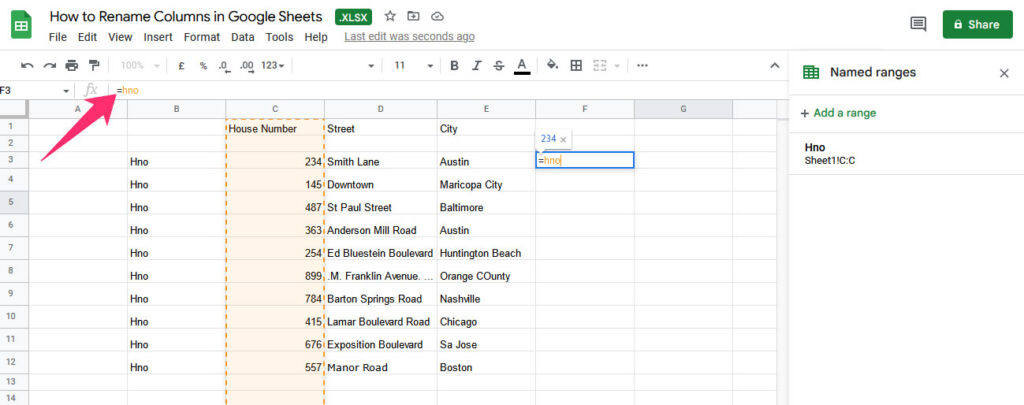
Naming columns in Google Sheets is not possible directly, but you can “rename them” by creating ranges. Below I have explained how you can create named ranges for columns.
How to Label Columns in Google Sheets Using Named Ranges
Step 1: Open the Google Spreadsheet in which you want to rename columns.
Step 2: Now click on Data from the Options Menu, and select Named Ranges.
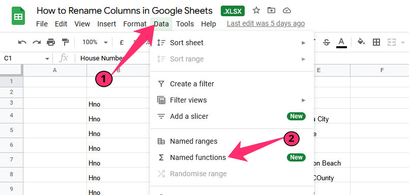
Step 3: A dialogue box will open on the right side of the screen. Click on Add a Range.
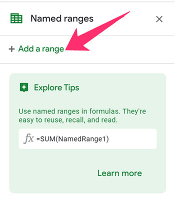
Step 4: Select the column that you want to change the name for.
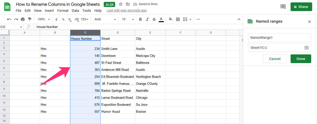
Step 5: Now enter your preferred name in the name range section. Make sure there is no space or other signs in the new name, as Google Sheets don’t support them.
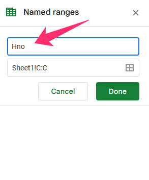
Step 5: Click on Done, and you have successfully renamed the column.
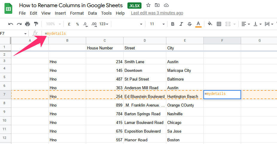
Step 6: Now, you can use this name when entering formulas in Google Sheets.
How to Create Column Headers in Google Sheets
If you want an alternative to column headers and want the column name visible while you scroll in the Google Spreadsheet, you can use the freeze feature. This function freezes the selected row, which shows you the column headers you want.
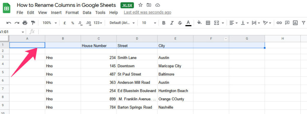
Step 1: Select the columns you want to create headers for.
Step 2: Click on View from the Menu bar option, and select Freeze.
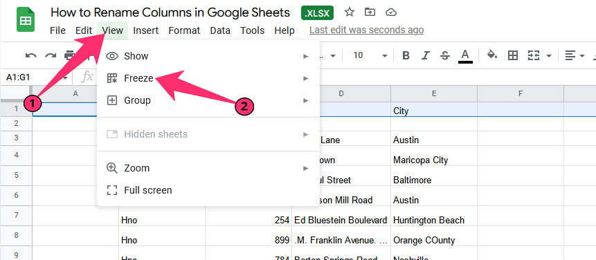
Step 3: Now choose Freeze 1 Row, and you are good to go.
Step 4: As you scroll down in the sheet, the selected columns will always be visible as headers.
PS. I wrote an entire article on how to keep a row fixed in google sheets so make sure you don’t miss it 🙂
How to Rename Rows in Google Sheets
Technically, you cannot rename a row in Google Sheets, but you can use the name ranges to easily assign a name to use the specific row in formulas.
Step 1: Click on Data from the menu bar, and select name ranges.

Step 2: Click on Add a Range, and then select the row you want to rename.
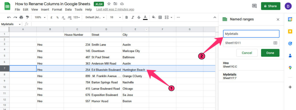
Step 3: Give the row a name of your choice, and click on Done.
Step 4: Now, you can use the new name in formulas to select the row you have renamed.
How to Rename Columns in Google Sheets Mobile App (iPhone, iPad, and Android)
At the moment of writing this tutorial, you cannot rename columns in Google Sheets using the mobile app. Additionally, the named ranges function works only on the PC version.
Final Thoughts
This detailed article on how to rename columns in Google Sheets has explained everything in detail. You can follow these steps to rename rows and columns and use them in formulas without confusion.
One thing to note is that the name of the column or row header won’t be visible on the spreadsheet.
Do you have any queries regarding renaming rows and columns in Google Sheets? Drop your questions in the comments section, and I’ll get back to you.
Stay tuned with us to become a master at using Google Sheets!
