Copy/pasting data from one spreadsheet to another is easy, but things can get daunting when you want to copy lookup tables.
For example, one spreadsheet might have details related to the products your company wants to sell with the UPCs and other information, while another spreadsheet might contain many sales.
In order to calculate the total sale, you’ll need to pull pricing from the product sheet to the log sheet. And to do it, you need to reference another spreadsheet tab or cell.
If you have some technical know-how of Google Sheets, type “=SheetName!A1 or =’ Sheet Number Two’!C5” to refer to data from another sheet.
Read on to understand how you can reference cells and tabs from another spreadsheet.
How to Reference Another Sheet in Google Sheets?
There are three methods you can use to pull data from another sheet in google sheets of a different spreadsheet. Below I have explained all three methods, and you can choose the one you think is most convenient.
Reference Another Sheet Using the IMPORTRANGE Function
The IMPORTRANGE function helps you pull cell and tab values from any sheet to the spreadsheet you want. However, to use this method, you’ll need the URL of the sheet you want to source the data.
- Open the Google Sheet you want to fetch data from and copy its link. Make sure to copy the link till “/” and leave the remainder. As you can see in the example below, copy the green part of the sheet link, and leave the red part.
https://docs.google.com/spreadsheets/d/1BXgz8b8BepdqsZQK_7yUImyZohl0euajxEEAKVBMyuc/edit#gid=0
- Now open the sheet where you want to pull the information and select a cell.
- Type =IMPORTRANGE(“URL”,”Sheetname!Cellrange”).
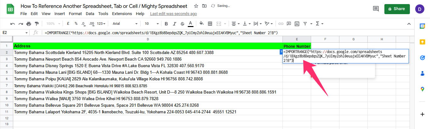
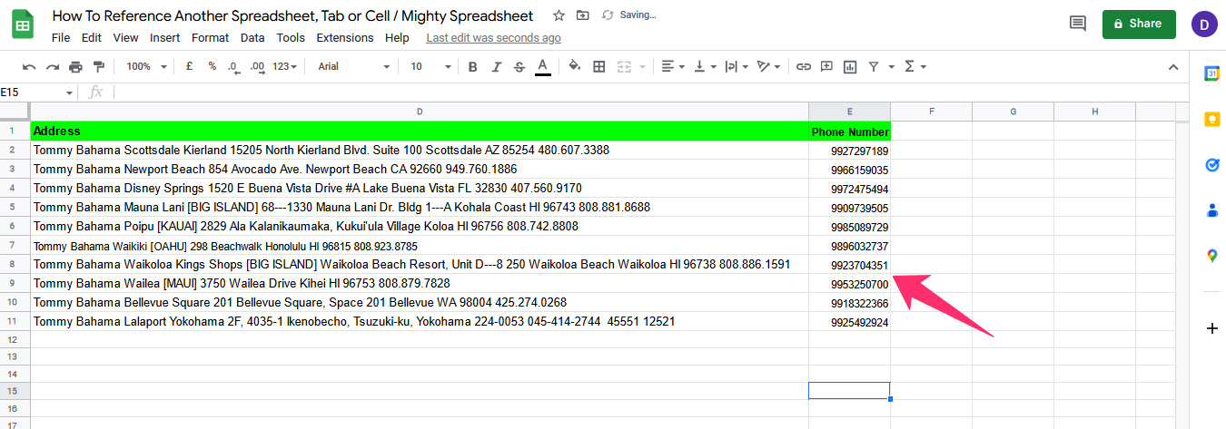
- Press Enter, and the data will be pulled to the spreadsheet.
How Link to Another Spreadsheet Using the HYPERLINK Method
Sometimes, you won’t need the data to be physically present in the sheet, so you can use a URL to link to the dataset you want. And when you click on the link, you’ll be automatically transferred to another spreadsheet with specific data.
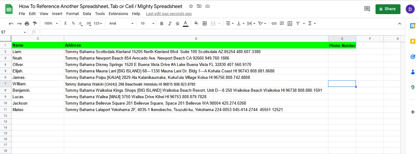
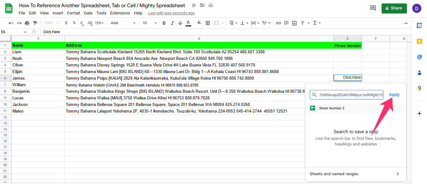
- Here is a spreadsheet where I want to add the phone numbers by referencing another spreadsheet that contains the phone numbers.
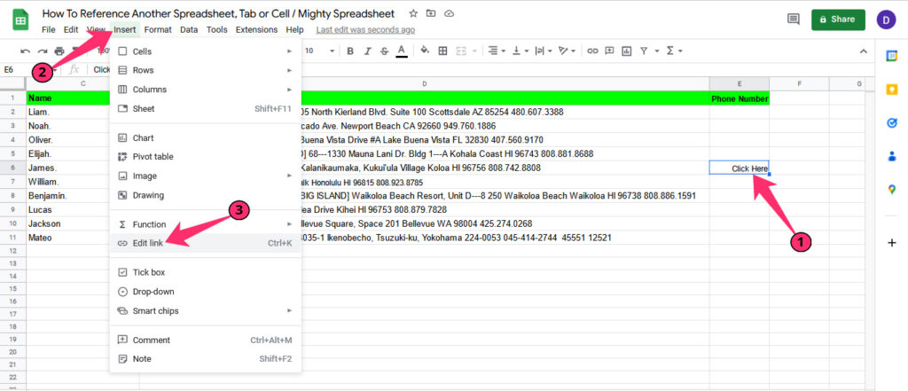
- I made a Click Here button by typing click here in a cell. Now I selected Insert and then Edit Link.
- I then pasted the link in the dialog box and clicked on Apply.
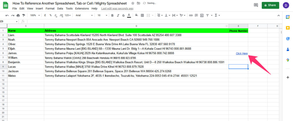
- When I click on the Click Here button, it takes me to the linked spreadsheet with the phone numbers.
How To Pull Data From Another Sheet Based on Criteria
If you want to pull specific data from one sheet to another, you can do it by defining criteria. The criteria help you set limits, and you only get the values you want.
The basic formula looks like: =FILTER(data_set,criterium1, criterium2,...)
- Data set: A range of cells you want to filter.
- Criterium: The criteria you want to filter the data set.
Here are the steps to pull data from another sheet based on the criteria:
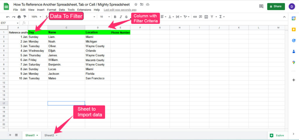
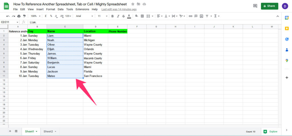
- The image attached below explains the “data to filter,” “column with filter criteria,” and “sheet to import data to.”
- Open the sheet where you want to import the data and select a cell. Now type
=filter('Source data'!CellRange,' Source data'!CellRange=" Filter Data")
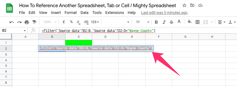
- I filtered the data by using “Wayne County” as the filter criteria, and it returned me with the result.
How to Reference Another Tab/workbook in Google Sheets?
If you want to reference a tab or workbook of the same spreadsheet, you can do it in two ways.
How to Import Data from Another Tab in Google Sheets
- Open the spreadsheet you want to import the data from and select the range of cells.
- Now go to another tab, and select a sell. Enter “
=Sheet name!Range of cells“
- Press Enter, and the data will be imported automatically.
Link to Another Tab in Google Sheets
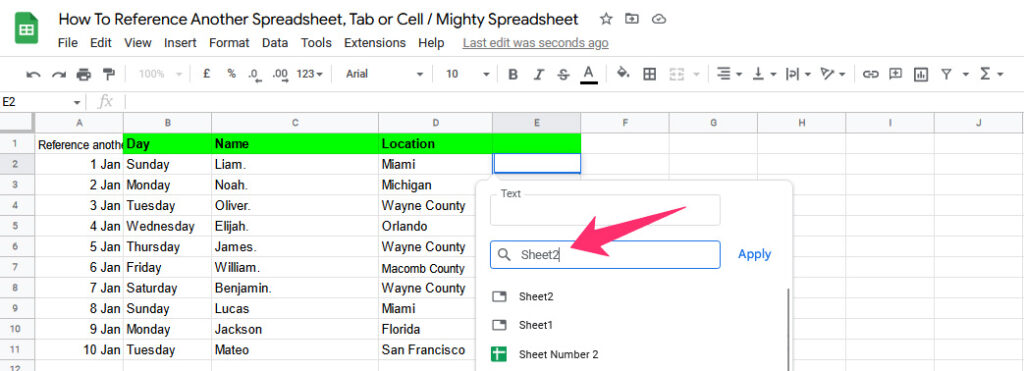
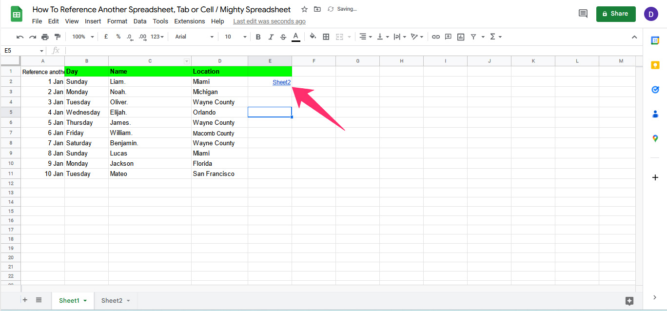
If you don’t want the data to appear physically on your sheet, you can link the tab in Google Sheets.
- Open the sheet, and select a cell. Right-click and choose Insert Link.
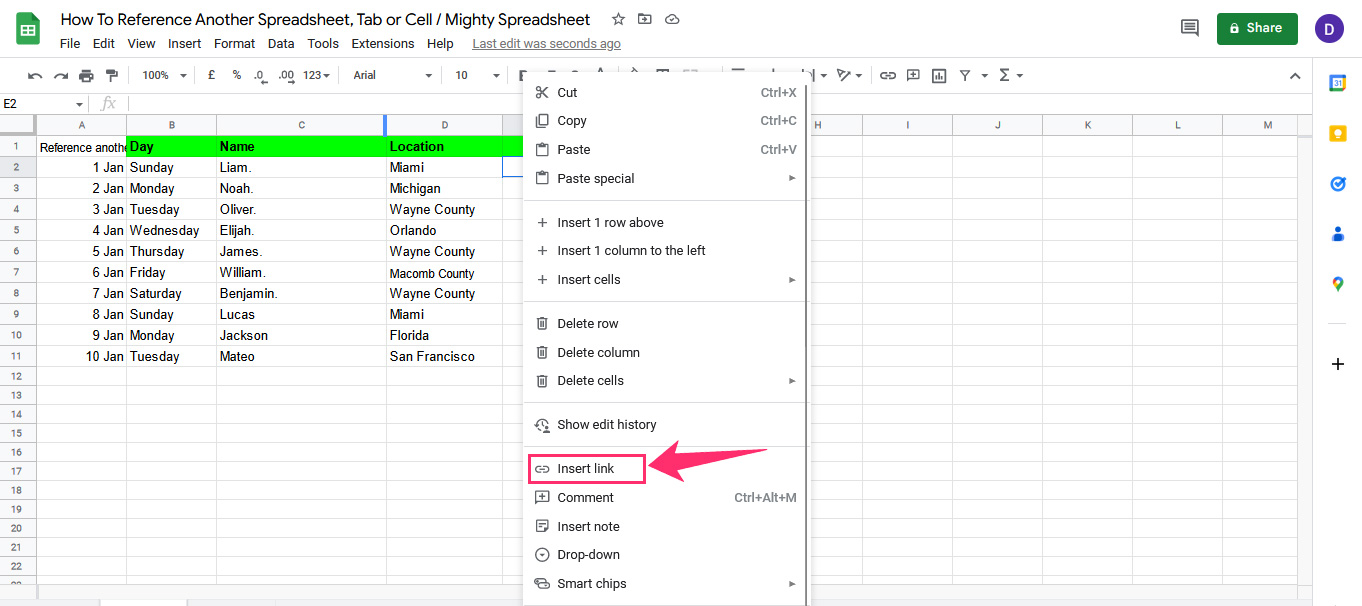
- Now enter the sheet name in the text box, and click on Apply.
- The link will be added to the cell, and when you click on it, you’ll be redirected to another tab or workbook.
How to Reference Another Cell in Google Sheets?
There are two ways to reference another cell in Google Sheets, depending on where you want to refer the cell from. Below I have covered both methods to help you refer to another cell within the same sheet and from a different sheet.
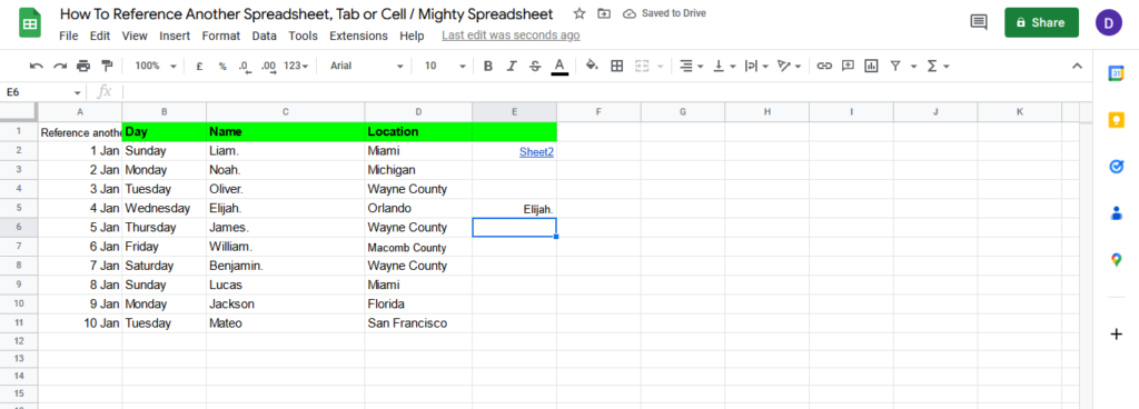
Method 1: Reference Another Cell in the Same Sheet
- Select an empty cell where you want to reference the cell data you want. Enter “
=Cell Number“
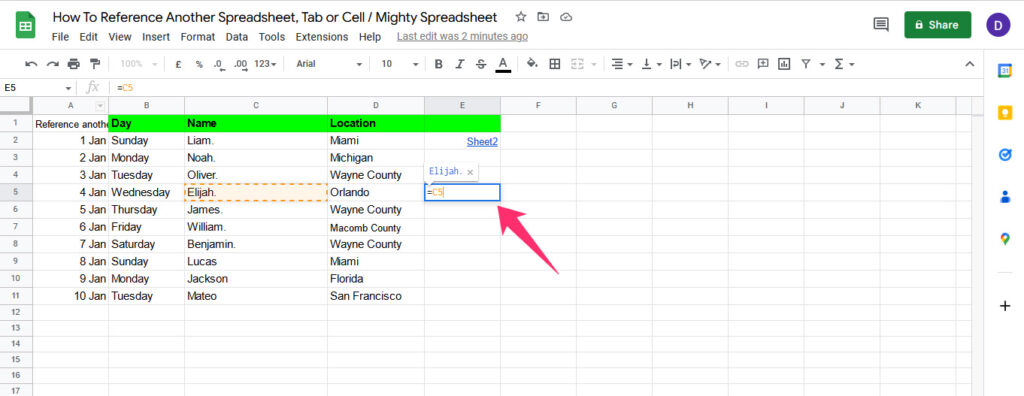
- Press Enter and the data from the referred cell will automatically appear in the selected cell.
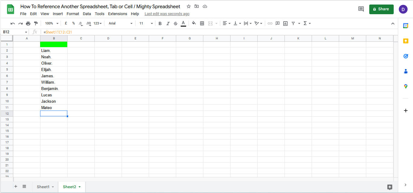
Method 2: Reference Another Cell from a Different Sheet
To reference another cell from a different sheet, you’ll need to use a formula: “=SheetName!CellAddress”.
Here’s a breakdown of what each part means:
- SheetName: This is the name of the sheet where the cell you want to reference is located. If you’re referencing a cell on the same sheet, you can leave this part out and just use an exclamation mark (!) to separate the sheet name from the cell address.
- “!” This is the exclamation mark that separates the sheet name from the cell address.
- CellAddress: This is the address of the cell you want to reference. It can be a single cell (e.g., A1) or a range of cells (e.g., A1:B10).
Here’s how the formula works:
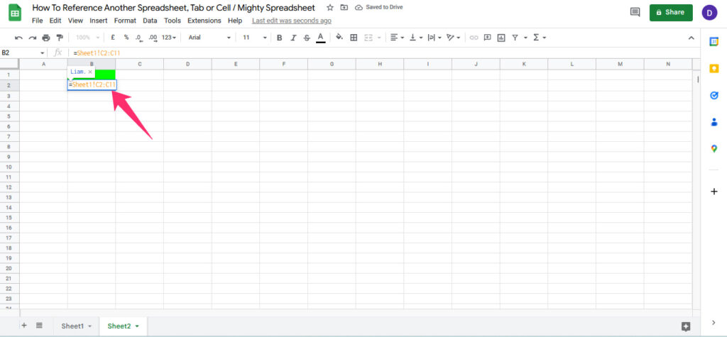
- Open the sheet and select a cell where you want to refer data from another cell. Type “
=Sheetname!Celladdress”.
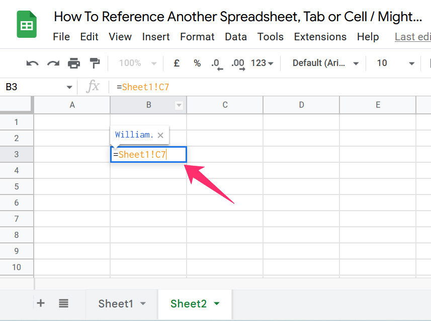
- Press Enter, and the data from cell C5 from Sheet 1 will be sourced to Sheet 2.
How to Import Data from Multiple Sheets Into One Column
You can use the IMPORTRANGE method to import data from multiple sheets into one column. However, you need to be specific about the formula since using multiple URLs can lead to errors and mistakes.
The simple formula of IMPORTRANGE for importing data from one sheet into the column is: =importrange("url_of_workbook," "data_range").
When you want to import data from multiple sheets, you can put multiple URLs into the formula by using a pair of braces and semicolons to separate each set.
Here’s how the formula should look:
={importrange(url1,range1);importrange(url2,range2);importrange(url3,range3)}.
You can even use IMPORTRANGE to import multiple sheets from a single spreadsheet into one column by using the formula:
={importrange(url,range1);importrange(url,range2);importrange(url,range3)}
How Can I Get Google Sheets to Auto-update a Reference to Another Sheet
It can be a daunting task to refresh your spreadsheet every time you make a change to it to reference it to another sheet. However, there is a hack that saves you from this trouble, and the referred data gets updated automatically.
- Open the spreadsheet, and click on File. Scroll down and select Settings.
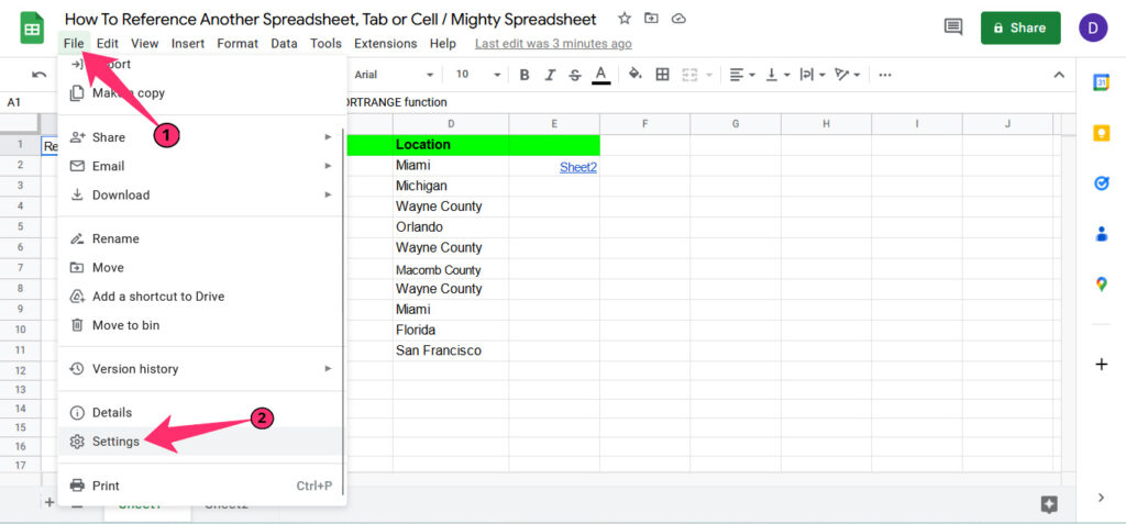
- Click on Calculation, and select the drop-down menu under Recalculation.
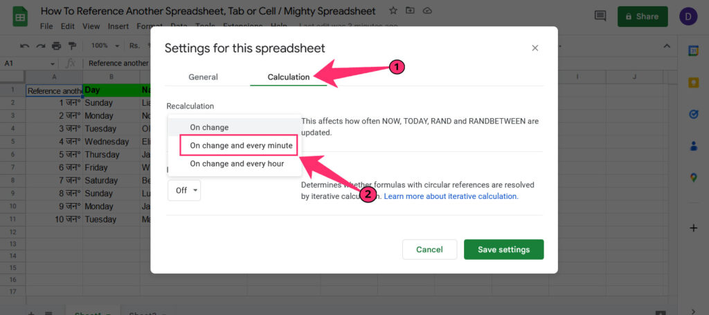
- Select On Change and Every Minute, and click on Save Settings.
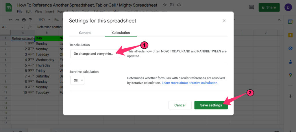
- This setting will activate the auto-update function, and the referred data gets updated automatically.
FAQs
Q: Can I reference a cell using its column and row number instead of its address?
A: Yes, you can reference a cell using its column and row number instead of its address in Google Sheets by using the INDIRECT function with the ADDRESS function. For example, =INDIRECT(ADDRESS(2, 3)) will return the value of the cell in the second row and third column (i.e., cell C2).
Q: How do I reference a named range from a different sheet?
A: To reference a named range from a different sheet in Google Sheets, you can use: “=SheetName!NamedRange”. Replace “SheetName” with the name of the sheet that contains the named range and “NamedRange” with the name of the range you want to reference. For example, if you have a named range called “SalesData” on a sheet called “Sheet2”, you would use the following formula to reference it from another sheet: “=Sheet2!SalesData”.
Q: How do I use a reference to a cell or range of cells in a formula that includes multiple sheets?
A: To use a reference to a cell or range of cells in a formula that includes multiple sheets in Google Sheets, you can use the formula: =SUM(Sheet1:Sheet3!SalesData).
This example formula adds up the values in the SalesData range on sheets Sheet1, Sheet2, and Sheet3. Replace “SalesData” with the name of the named range you want to reference and “Sheet1” and “Sheet3” with the names of the sheets you want to reference.
Final Thoughts
I hope this guide on how to reference another spreadsheet, tab, or cell in Google Sheets has helped you source data on the go. Make sure to use the right formula to get the data imported quickly and without any errors.
Do you have any questions regarding importing data from another spreadsheet, cell, or tab? Leave your queries in the comments section, and I’ll get back to you at the earliest opportunity.
Stay tuned with us for more such posts and become a master at using Google Sheets.