Concatenate Function In Google Sheets (Join Strings Like A PRO!)

At times, you need to join (not add) two or more cells in your spreadsheet to have specific outputs. And through the “Concatenate” function in Google Sheets, you can do that in seconds. You can easily join multiple strings with this one.

You can join strings in Google Sheets with “Ampersand (& sign),” “CONCAT,” “CONCATENATE,” and “JOIN” functions. While “&” will give you basic output, the other three functions are versatile and can be implemented for an entire cell range with delimiters.

However, all these four functions (and some additional ones) have their advantages and limitations. You will get the best output while using specific functions depending on your requirement. Let’s check out my methods (with live examples)!

How To Concatenate Strings In Google Sheets?

You can easily join values and even texts in Google Sheets. And there are four different methods available that have specific purposes. So, I’m going from the easiest to pro-level methods.

Method 1: Use The “&” Function

Let’s start with a very basic function that may serve your purpose if you don’t have a complex sheet. For simple operations, the “&” function can join two cells with text or values. Here goes the detail to combine strings.

• Step 1: Select an empty cell where you need to join strings in Google Sheets to get the final output.
• Step 2: Click on the “Functions” tab and enter the “=<first cell>&<second cell>” formula.

• Step 3: Hit enter to get the output. 

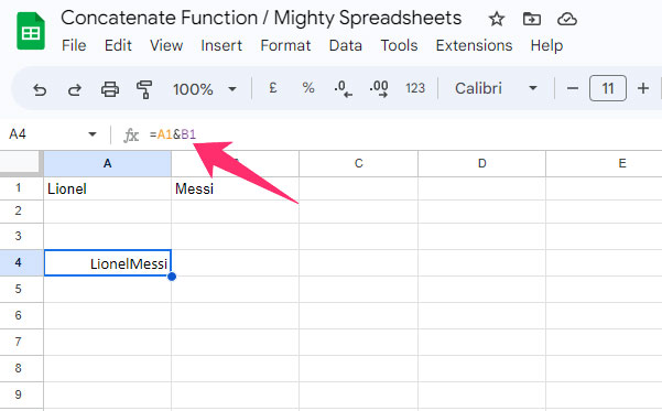
Explanation: I have “Lionel” in the A1 cell and “Messi” in the B1 cell, and I want the final output in the C1 cell. 

So, I need to select the C1 cell first and then enter the “=A1 & B1” formula. It will give me the final output as “Lionel Messi” in the C1 cell.

Limitations: All the basic things have their limitations, and so does this “&” function. Although it is useful in some instances, it is not even versatile.

• Only useful for simple operations where cells don’t have complex or alphanumeric values.
• Very prone to error, especially if you are using complex data.
• You can join as many cells as you want. But using more cells will cause more errors.

Note: Do you know that it is now possible to remove duplicate data and values from your spreadsheet using simple functions? Do check out my latest guide on removing duplicates in Google Sheets very efficiently.

Method 2: Use The “CONCAT” Function

The CONCAT function is a simple command that lets you join two strings (text & text or number & number) in Google Sheets. It is a reliable function for combining text in google sheets. And the steps are pretty easy!

• Step 1: Open Google Sheets and select an empty cell where you need the output.
• Step 2: Click on the “Function” tab (fx).
• Step 3: Put the “=CONCAT(<first cell>,<second cell>)” formula.

• Step 4: Hit the enter button to get the joined output in your desired cell.

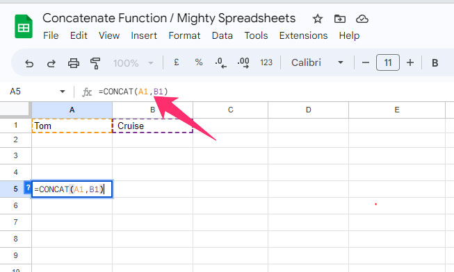
Explanation: Let’s say I have “Tom” in the A1 cell and “<space>Cruise” in the B1 cell, and I need to join them to get the final text output in the C1 cell. 

So, I need to select the C1 (output cell) first and enter the CONCAT function. My formula will be “=CONCAT(A1,B1),” where the final output will be “Tom Cruise.”

You can do the same thing with values, but it will not add the value but will display them together as a single value. 

Let’s say I have “5” in the A2 cell and “6” in the B2 cell, and I need the output in the C2 cell. The final output will be “56” after using the CONCAT function.

Limitations: CONCAT is a very basic function that doesn’t give you many options to moderate or to collaborate with other functions. And it has several downsides.

• You can only join two strings with this function.
• This function cannot include a “space” in between the strings.
• You can only join but can’t add values.

Bonus: Google Sheets now gives you the option to collaborate and share your spreadsheet in real-time. Check out my latest guide to sharing and collaborating in Google Sheets to know more.

Method 3: Use The “CONCATENATE” Function

The “CONCATENATE” function can join multiple variables. It is pretty effective when you want to combine text from two or multiple cells in Google Sheets, as other basic functions will not give you this option. Here goes the method!

To join two cells (With or without delimiter):

I have “Cristiano” in the A1 cell and “Ronaldo” in the B1 cell, and I want to get the final output in the C1 cell. So, the steps will be,

• Step 1: Select an empty cell (here it is C1).
• Step 2: Click on the “fx” tab and enter the “=CONCATENATE (A1,B1)” formula.

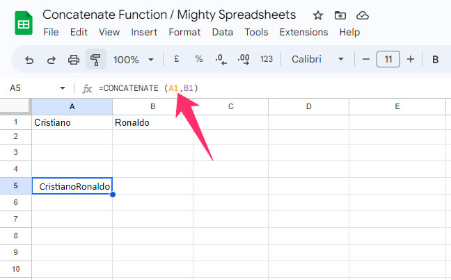
• Step 3: Hit the enter button, and the final output will be “CristianoRonaldo” in the C1 cell.

You can see that the final output delivers without space. But I want to concatenate with space between these two strings. To do that, we will use a delimiter with this function. 

• Step 1: Enter the “=CONCATENATE (A1,“ ”,B1)” formula in the function tab.

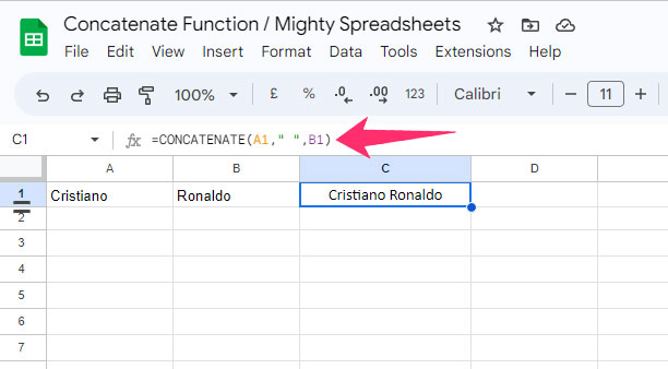
• Step 2: Hit the enter button, and the final output will be “Cristiano Ronaldo” in C1.

I’m showing you this example with just text values. But you can do the same thing with any numeric or alphanumeric value. 

It also gives you the freedom to join a text value with a number value. And you can use as many cells as you want in this formula.

To join multiple cells:

Let’s say I have “Portuguese” in A1, “Footballer” in B1, “Cristiano” in C1, and “Ronaldo” in D1. And I want to get the final output in the E1 cell.

• Step 1: Select an empty cell (it is E1 in this case).
• Step 2: Click “fx” and enter the “=CONCATENATE (A1," ",B1," ",C1," ",D1)” formula.

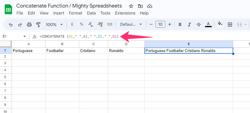
• Step 3: Hit enter, and the final output will be “Portuguese Footballer Cristiano Ronaldo” in the E1 cell.

It’s time to make this even more complex. I have “Cristiano Ronaldo” in A1 cell, “Al Nassr FC” in B1, and “2023” in C1. But I want to use the “Plays For” delimiter between A1 and B1 and the “Since” delimiter between B1 and C1.

• Step 1: Select the output cell (it is D1 here).
• Step 2: Click “fx” and enter the “=CONCATENATE (A1,“ Plays For ”,B1,“ Since”,C1)” formula.

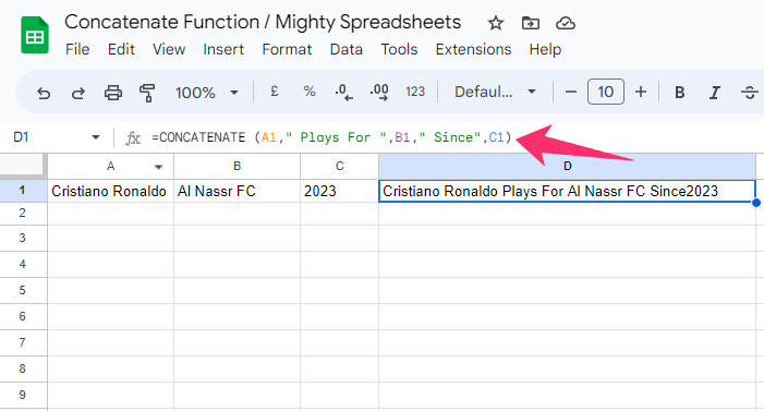
• Step 3: Hit the enter button, and the final output will be “Cristiano Ronaldo Plays For Al Nassr FC Since 2023” in the D1 cell.

Note: Like the “Ampersand” function, the “CONCATENATE” function also can’t produce space in between words. So, to adjust that, I’ve used a delimiter with spaces on both sides (“<space>Plays For<space>” instead of “Plays For”).

To join multiple cells but to get output in separate lines (with line breaks):

I have “LeBron James” in the A1 cell, “Nikola Jokic” in the B1 cell, “Luka Doncic” in C1, and “Jayson Tatum” in D1. And I need output like a team roaster while having each player in separate lines in the E1 cell.

We will now combine the “CONCATENATE” function with the “char(10)” function while also using the ampersand to get the final output.

• Step 1: Select the output cell (here it is E1).
• Step 2: Click on the “fx” tab and enter the “=CONCATENATE(A1 &char(10),B1 &char(10),D1 &char(10),D1)” formula.

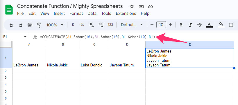
• Step 3: Hit enter, and the final output will come with line breaks after each player in the E1 cell.

You can even add date functions in this final output string by using the “TEXT(<input cell>, “MM/DD/YYYY” formula. I also have a separate guide on how to use the “Date” function in Google Sheets. Do check it out to know more!

Method 4: Use The “JOIN” Function To Concatenate With Separator

Google Sheets offer another function called “JOIN” that can also concatenate cells with two separate values into one. It can also add delimiters of various kinds while delivering the final output. 

To join cells (With or without delimiter):

Let’s say I have “Thomas” in the A1 cell, “Edward” in B1, “Patrick” in C1, and finally, “Brady” in D1. I need the full name of Tom Brady as an output in the E1 cell, where all the words will be separated by a space.

• Step 1: Click on the empty cell where you need the output (here, it is E1).
• Step 2: Click on the “fx” tab and enter the “=JOIN (” “,A1,B1,C1,D1)” formula.

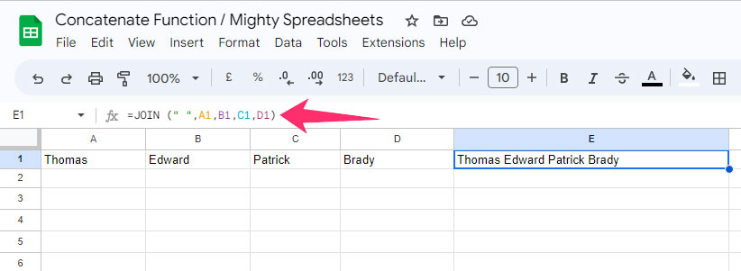
• Step 3: Hit enter, and the final output will be “Thomas Edward Patrick Brady” in the E1 cell.

Now, I have “Fiat” in the A1 cell, “Ford” in B1, “Chevrolet” in C1, and “Toyota” in D1. And I need the output in the E1 cell where all these words will be placed side by side concatenated with a comma. The steps will be,

• Step 1: Click on the output cell (in this case, it is E1).
• Step 2: Click on “fx” and put the “=JOIN (", ",A1,B1,C1,D1)” formula.

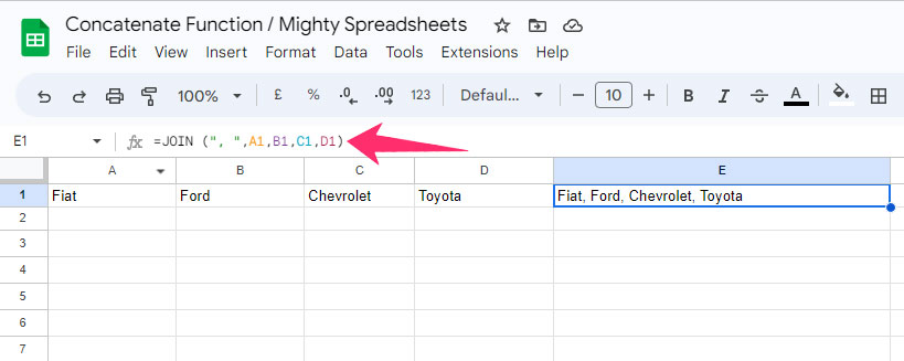
• Step 3: Hit enter, and you’ll get the final output “Fiat, Ford, Chevrolet, Toyota” in the E1 cell.

Here you can see that I’ve used the “,<space>” delimiter in this formula while using A1 to D1 as the input cells. I used a space after the comma sign in the delimiter because I needed a space after each comma in the final output.

To join cells (With line breaks):

This time, I have “Aaron Rodgers” in the A1 cell, “Peyton Manning” in B1, “Jerry Rice” in C1, and finally “Brett Favre” in D1. And I need the output in the E1 cell where all the NFL players will be displayed in each line.

• Step 1: Click on E1 (the output cell).
• Step 2: Click on “fx” and put the “=JOIN(CHAR(10),A1:D1)” formula.

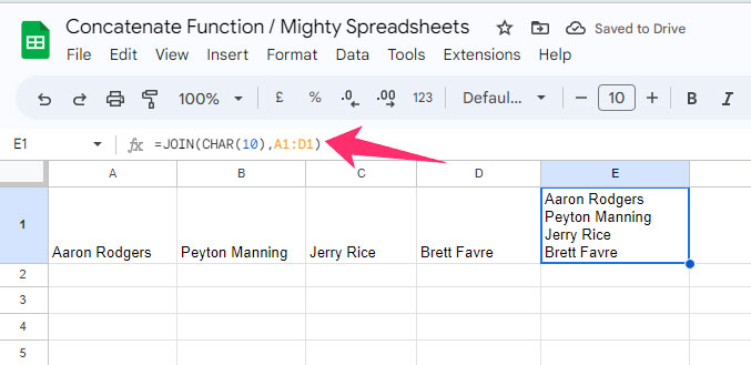
• Step 3: Hit the enter button, and players separated by line breaks will appear in E1.

I’ve used the “CHAR(10)” function as the delimiter here. And without giving individual cells, I placed the complete cell range with the “A1:D1” formula, which automatically takes inputs from A1 to D1 cells.

Bonus: You should filter your data first on Google Sheets if you are working with a complex structure. The steps are easy, though! And I’ve given a brief insight on how to filter data in Google Sheets in my latest blog.

How To Combine Text And Formula In Google Sheets?

If you don’t want just to join strings but need an output by using a formula, you can even do that in Google Sheets by using the “=CONCATENATE(<formula>,” <string/cell range>”)” formula. And the steps are also very easy.

Join text and formula:

I have “100” in A1, “200” in A2, “300” in A3, and “400” in A4. And I need to have an output as the sum of these values with “Dollars” written on it in A5. So, the steps will be,

• Step 1: Select the empty output cell (here it is A5).
• Step 2: Click on “fx” and enter the “=CONCATENATE(SUM(A1:A4),” miles”)” formula.

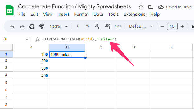
• Step 3: Hit the enter button to get the “1000 miles” output in the A5 cell.

If you don’t have a cell range but only want to work with two, you can use “<First cell>,<second cell>” in the cell range. And not just an addition; you can even put complex formulas in the first command.

Join formula and delimiters:

Again, I have “100” in A1, “200” in A2, “300” in A3, and “400” in A4. But this time, I want to have an output with “we received” in the prefix and “dollars” in the suffix while all the values are added. I’m making some minor changes to this formula.

• Step 1: Click on the output cell (here it is A5).
• Step 2: Click “fx” and enter the “=CONCATENATE(“We received ”,SUM(A1:A4),” dollars”)” formula.

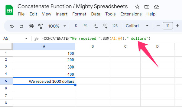
• Step 3: Hit the enter button, and you’ll get the output in the A5 cell.

Explanation: You can see that I’ve used two <spaces> in this formula. First, I’ve included a space after the “We received” part because I want to have a space in front of the total value. And then, I placed another space in front of “dollars” because I wanted to separate the value and texts after that.

Bonus: You can now easily use named ranges in your existing Google Sheets to fetch your data more efficiently. And to know more, check out my latest guide on using named ranges in Google Sheets.

Final Note

If you want to use just two cells that contain either value or text, you can simply use the ampersand (&) function in Google Sheets. Although this formula is the easiest, it is quite prone to errors, and you can’t incorporate this one in complex data.

So, if you have complex data and need to join multiple strings, even with formulas, you need to use the “CONCAT” or the “CONCATENATE” functions. You can even use the “JOIN” function as well. These three formulas are much more versatile than ampersand and can be a lifesaver in complex data structures. 

Some Questions You May Still Have

How to concatenate double quotes in Google Sheets?

You can use delimiters/separators inside double quotes while using the “CONCATENATE” function in Google Sheets. But if you are using any text as a delimiter, you also need to insert a space inside the double quotes, depending on where you want it.