How To Remove Duplicates In Google Sheets? (5 Solutions)

If you work with a huge amount of data, it’s highly likely that you have duplicate values in your worksheet.

It’s nothing to worry about because you can remove them quickly, but did you know there are many ways to do it?

You can use the “Remove Duplicates” feature under the “Data Cleanup” option.

You can also dedupe with “UNIQUE” and “QUERY” functions.

You can even use a 3rd party extension to remove all the duplicates from your sheet.

Let’s now focus on the best option to make your Google Sheet free from duplicates.

How To Delete Duplicates In Google Sheets? – 5 Working Methods That I Use

If you are wondering how to find and delete duplicates in Google Sheets, you need to know that there are at least 15 different methods to dedupe.

In this article, I’ll focus on the five ones I like the most and are suitable for newbies.

Method 1: Remove Duplicates Using The “Data Cleanup” Feature

This is the easiest and probably fastest way to eliminate duplicates in Google Sheets. This is what you need to do:

Step 1: Click any of the cells in your sheet and click on the “Data” option in the header menu.

Step 2: Hover your mouse over“Data Cleanup” and click on the “Remove Duplicates” option.

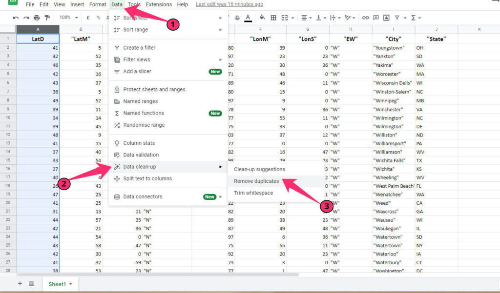
Step 3: Once you get a selection menu, tick the “Select all” option to check the entire sheet.

Step 4: Alternatively, you can choose any column (if you need to remove duplicates from specific columns).

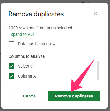
Step 5: Click on the “Remove duplicates” button.

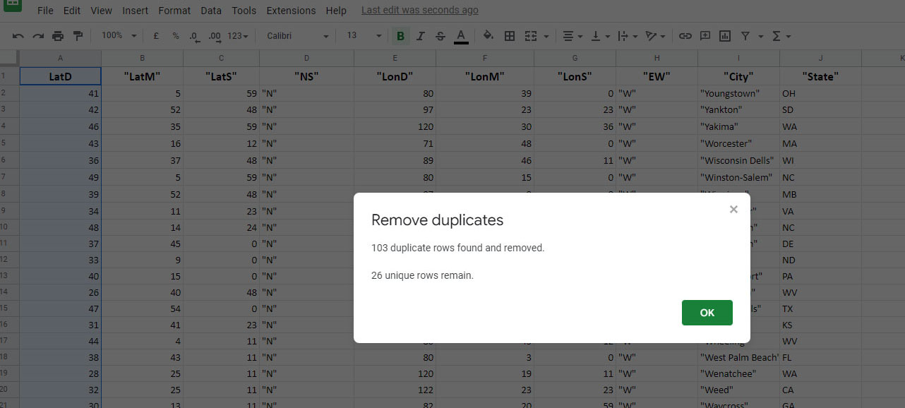
Step 6: Wait until you get a summary of deduping and click on the “OK” button.

Beneficial For: This method will be a great solution if you use Google Sheets for invoicing or bookkeeping, where you must delete duplicates in an entire worksheet.

Method 2: Get Rid Of Duplicates Using The “UNIQUE” Function

By using the “UNIQUE” function, you can easily remove duplicates from a selected data range and make it easier to work on large data sheets.

Here are the steps you need to follow to dedupe with this method:

Step 1: Select a free cell to input the function

Step 2: Type in the function command =UNIQUE(your_data_range)

In the example below, we will select all entries from B6 to G24. That’s why our formula will look like this: =UNIQUE(B6:G24)

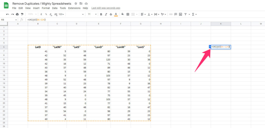
Step 3: Once executed, you can see your entire data range but with fewer rows. The new data will start from the place where you entered your function. (In my case, it started from K6)

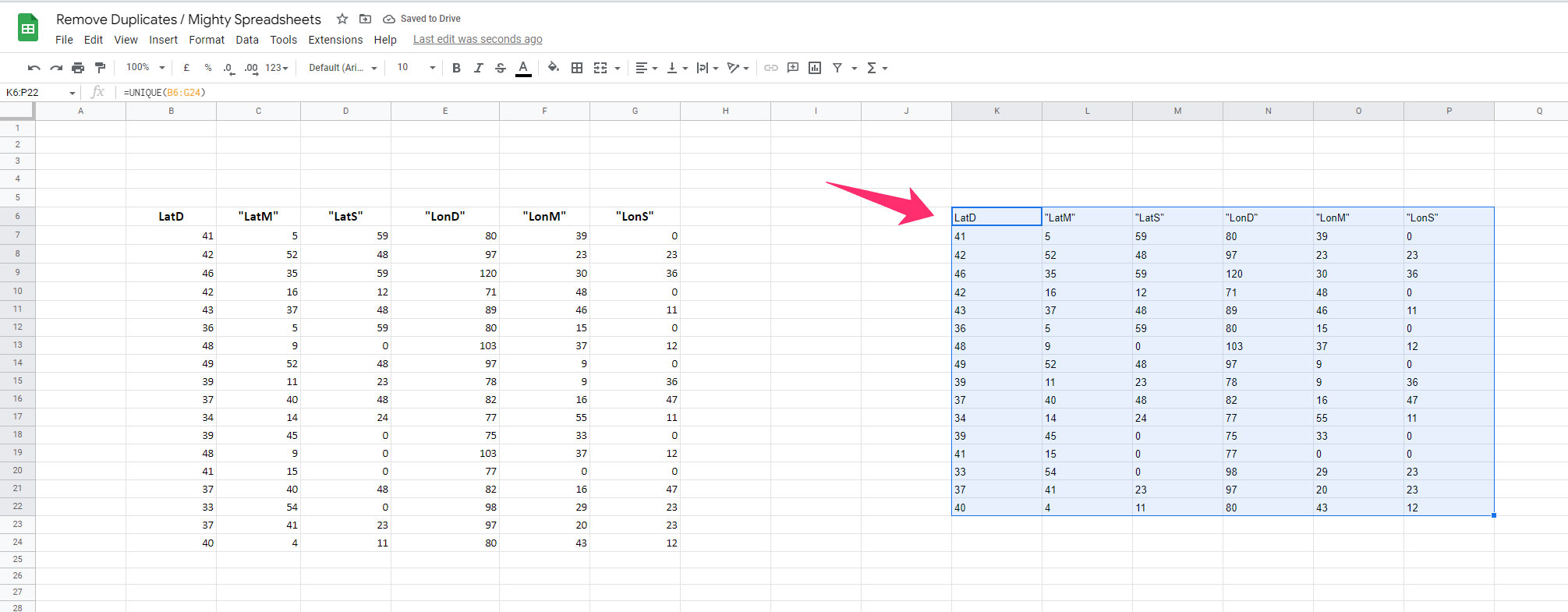
Step 4: Select the new unique columns and replace your previous data range containing duplicates.

This method is particularly helpful for working with a specific data range.

It will not be a good option if you want to dedupe the whole sheet, as it will create a new data range.

TIP: If you want to work on specific data rather than an entire sheet, you can filter data in Google Sheets.

Method 3: Remove Duplicates Using The “QUERY” Function

We will now move to a more advanced function to eliminate duplicates in Google Sheets and use the QUERY function.

But first, we will name our data range, so it’s easier to reference it in our formula.

(You can read this article if you want to learn how to use named ranges in Google Sheets)

Step 1: Press the “Ctrl + A” buttons (For Windows) or “Cmd + A” buttons (For Mac). (Alternatively, you can “Shift + Click” to select a specific range of data in your sheet)

Step 2: Click on the “Data” option on the header menu and find the “Named ranges” menu item.

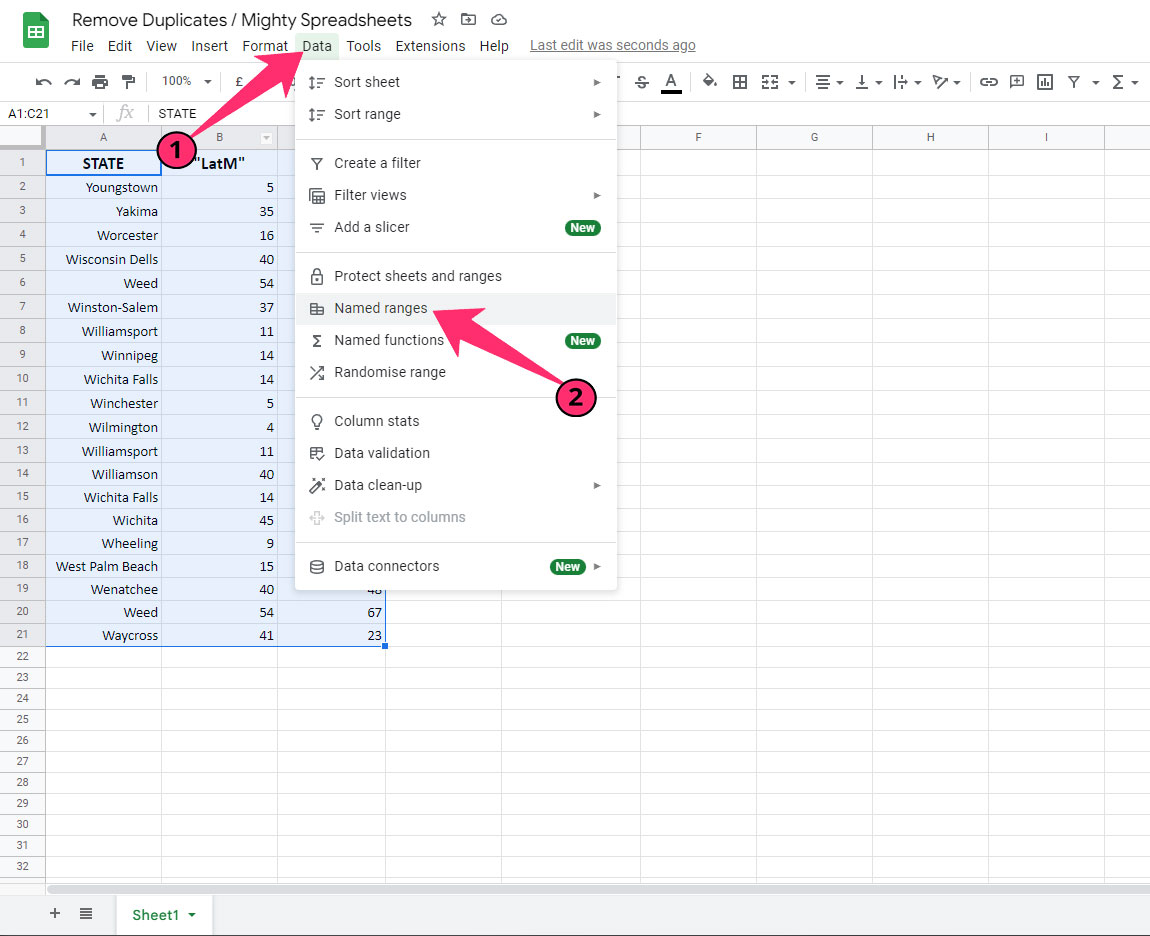
Step 3: Give it a suitable name once the naming panel appears on the right toolbar. (I’m using “GSdata” in my case)

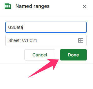
Step 4: Save the named range by clicking the “Done” button.

Step 5: Now, click on an empty cell. (In my case, it is E1)

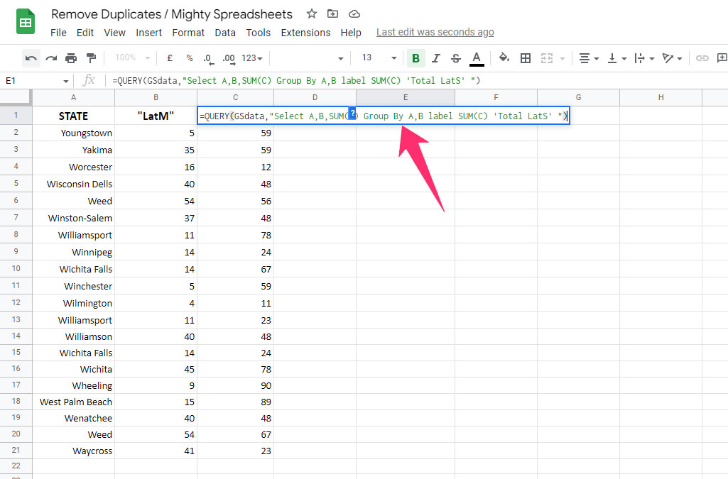
Step 6: Use the “GROUP BY” clause and create a function on that cell by using the “=QUERY(<named range>, “Select A,B,SUM(C) Group By A,B label SUM(C) ‘<the name you want to use in the last column’ “) formula.

Step 8: You can now see a new data range starting from your function cell (In my case E1), but with lesser rows.

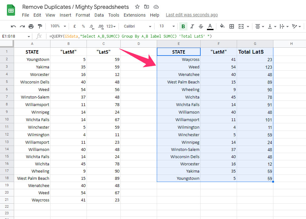
My Formula: In my case, I’m using “GSdata” as the range name and “Total LatS” in the last column. So, the formula will be =QUERY(GSdata, “Select A,B,SUM(C) Group By A,B label SUM(C) 'Total LatS')

Explanation Of My Execution:

• I have selected the first two columns (A & B) to remove duplicates from them and then give the total output value in the C column that I named “Total Output” in the formula.
• If you want to select more columns, adjust the formula accordingly.
• You can also use different outputs by replacing “SUM” with other functions, such as “AVERAGE” or “COUNT.”

Method 4: Eliminate Duplicates Using Pivot Tables

Removing duplicates in Google Sheets is also possible by using pivot tables. They are very flexible and quite simple to use. Here’s what you need to do:

Step 1: Select the data range you want to work with and click on the “Insert” option in the header menu.

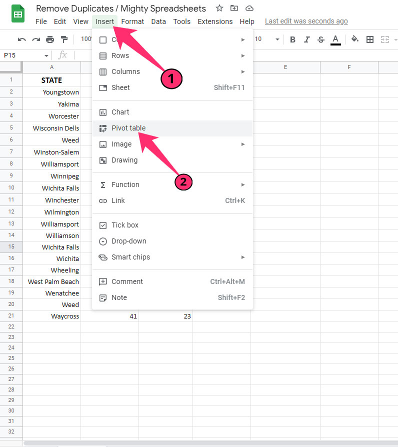
Step 2: Click on the “Pivot Table” option.

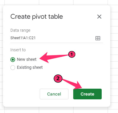
Step 3: Once you get a new pivot table option, select “New Sheet” and click on the “Create” button.

Step 4: After being redirected to a new page, navigate to the “Pivot table editor.”

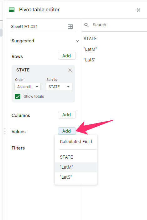
Step 5: Click the “Add” button next to the “Rows” tag.

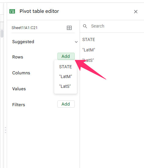
Step 6: Select the desired column name from the drop-down menu.

Step 7: Click on the “Value” option and choose the same or another column.

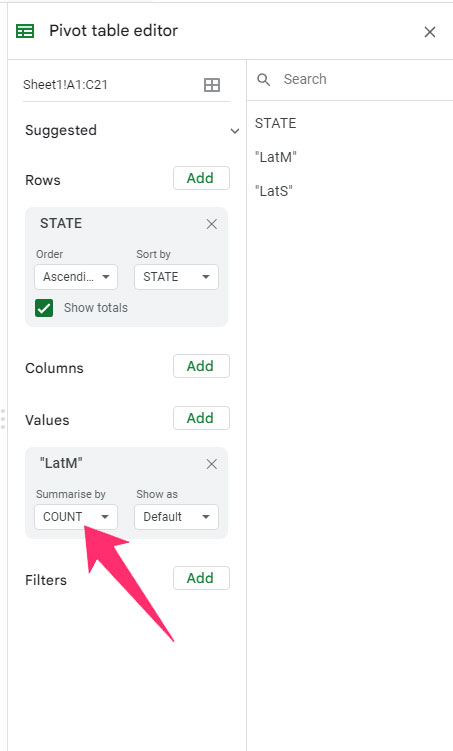
Step 8: Click on the drop-down menu below the “Summarize by” option.

Step 9: Select “COUNT” (if it contains numbers only) or “COUNTA” (if it contains text).

Step 10: Now, navigate to your created pivot table and select the second column (which has COUNT or COUNTA function).

Step 11: All those rows with a value of more than 1 have duplicates (E.G., if it is showing 2, then there are two duplicates etc).

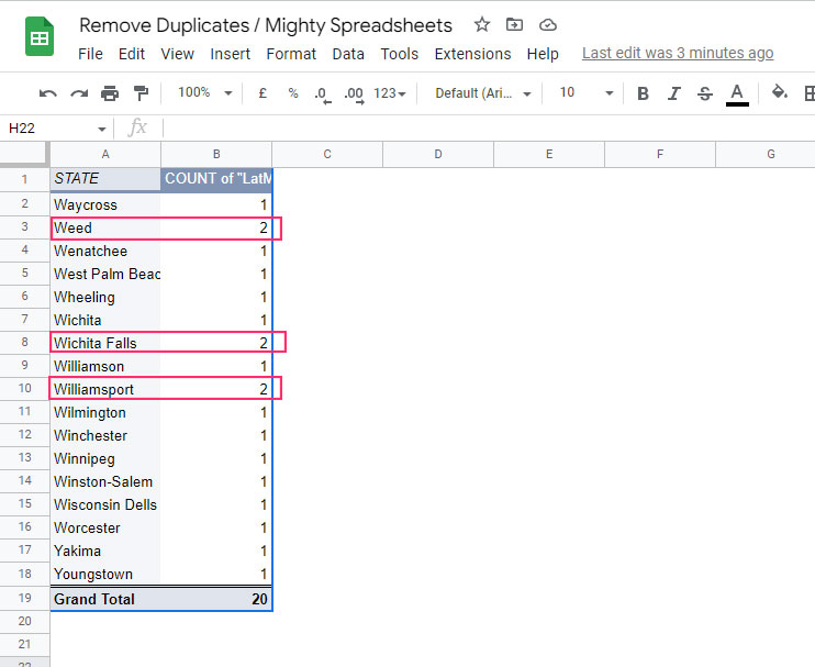
Step 12: Navigate to the main sheet and delete all the duplicates that you have traced in the pivot table.

Method 5: Remove Duplicates Using TheAblebits Add-on

I’m not a fan of installing addons for every operation you must perform, but the Remove Duplicates by AbleBits addon can help you with more complex examples if you are stuck.

Here are the steps you need to follow to install and use the extension:

Step 1: Open the sheet from which you want to eliminate duplicates and click on the “Extensions” option in the header menu.

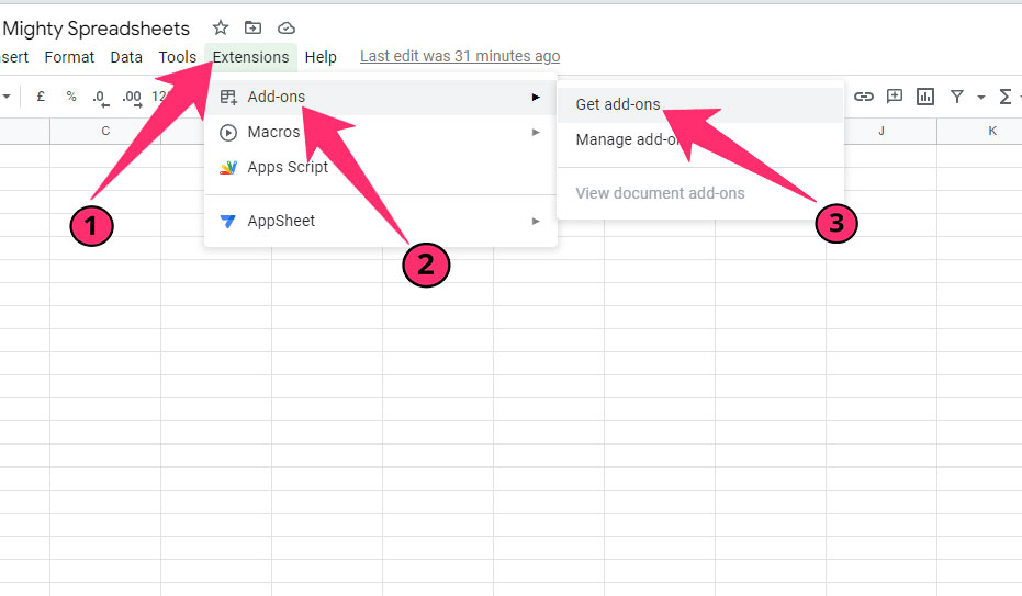
Step 2: Hover your mouse over the “Add-ons” option and click on the “Get add-ons” option.

Step 3: Once the “Google Workspace Marketplace” launches, type “Remove Duplicates” in the designated search field and hit enter.

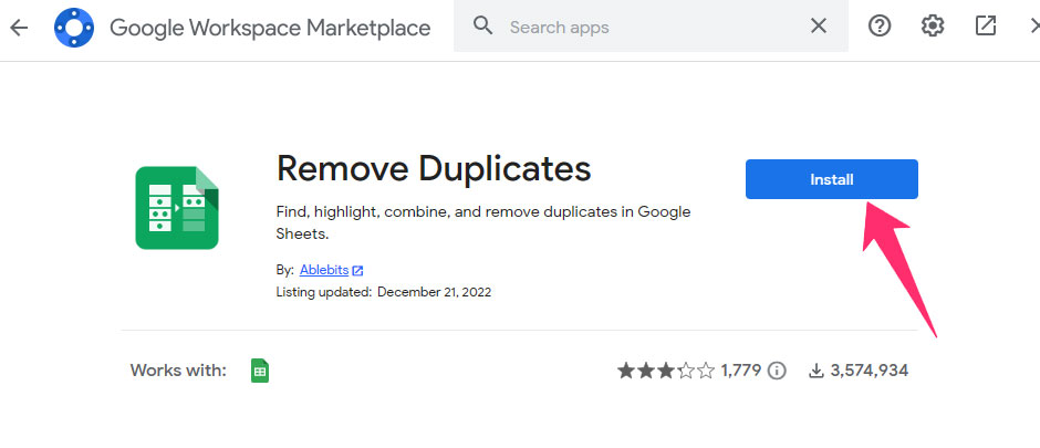
Step 4: Click on the “Remove Duplicates” preview; once redirected, click on the “Install” button.

Step 5: On the on-screen prompt, click the “Continue” button and select your Google account to proceed.

Step 6: Click the “Allow” button until it adds to your Google Sheet.

Step 7: Once completed, click on the “Done” button.

Step 8: Now, navigate to your main sheet and select the data range.

Step 9: Click on the “Extensions” and then on the “Remove Duplicates” option.

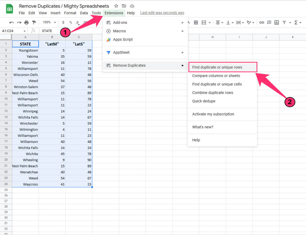
Step 10: Click on the “Find duplicate or unique rows” option from the new menu.

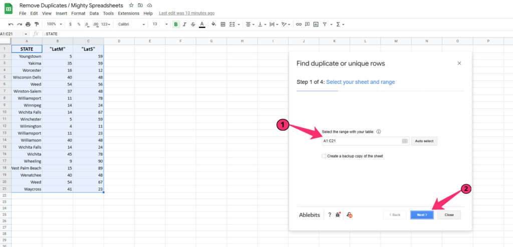
Step 11: After being redirected to a step-by-step prompt, insert the data range in the “Select the range with your table” option and click the “Next” button. (Tick on the “Create a backup copy of the sheet” option to save a backup file)

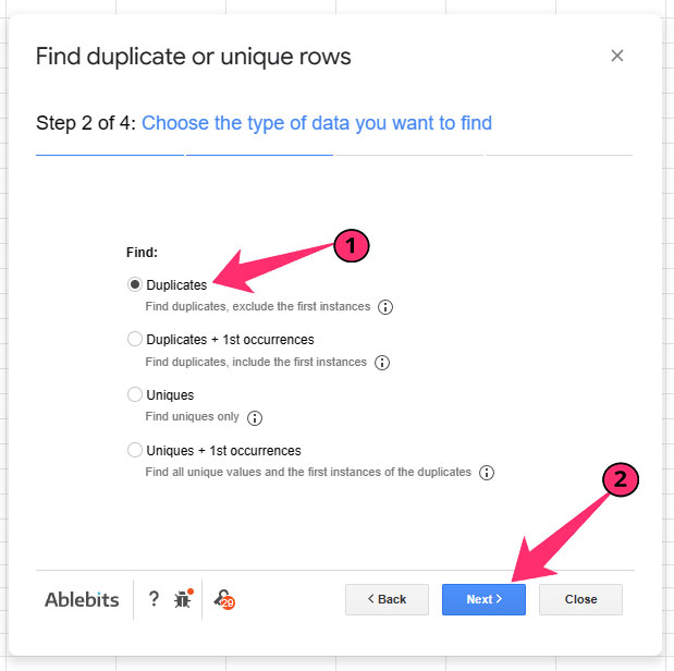
Step 12: On the second page, click on the “Duplicates” option and then on the “Next” button.

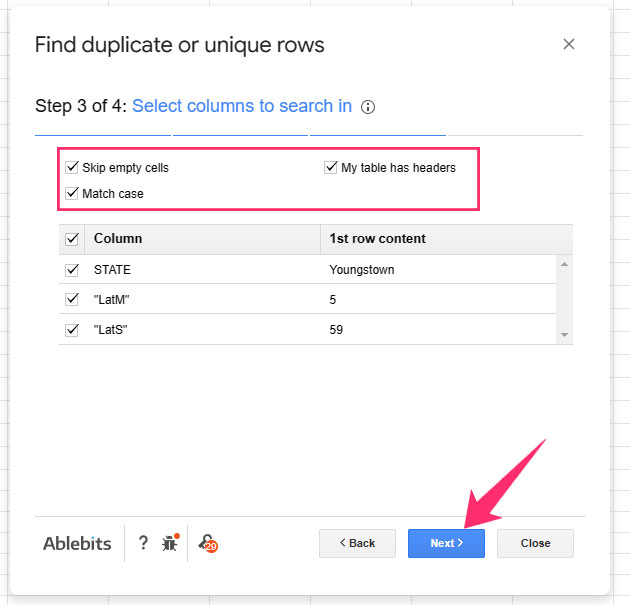
Step 13: Tick on the “Skip empty cells” and “Match Case” option, and then tap on the “Next” button. (You can also tick on the “My table has headers” option if the data range has it.)

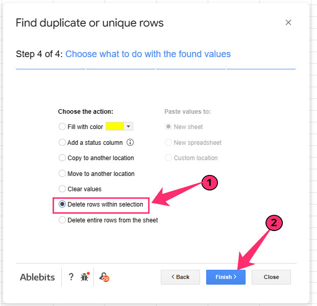
Step 14: On the fourth page, tick the “Delete rows within selection” option and then on the “Finish” button.

NOTE: The “Remove Duplicates” add-on by AbleBits is a paid extension that comes with a free trial. You can easily use the trial version for deleting basic duplicates. But you may need to purchase a subscription if you need advanced controls.

How To Remove Duplicates In Google Sheets Mobile App (iPhone, iPad, Android)?

There’s no option to do the “Data Cleanup” when using Google Sheets mobile app. On top of that, you cannot do much if you have iPhone or iPad.

However, there’s good news for you if you own an Android phone, as a workaround will help you. It will use conditional formatting to highlight the duplicated entries that you can delete manually.

Here are the steps to follow:

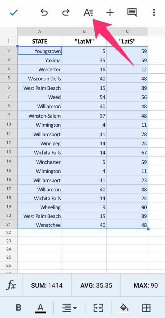
Step 1: Select the range of cells where you want to look for a duplicate.

Step 2: Tap on the “Format” button and then on the “Conditional formatting” option.

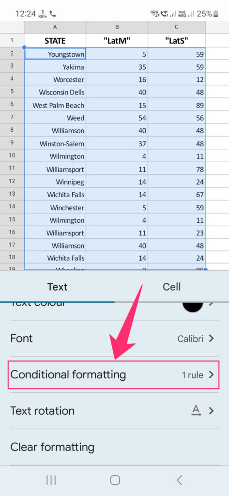
• Step 3: Navigate to the drop-down menu under the “Format cells if…” option (under “Format rules”).

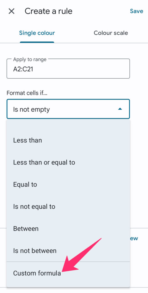
• Step 4: Scroll down the drop-down menu options and tap on the “Custom formula” option.
• Step 5: To highlight just the column having duplicate, put the “=COUNTIF($A$1:$A1,A1)>1” formula in the “Value or formula” field.

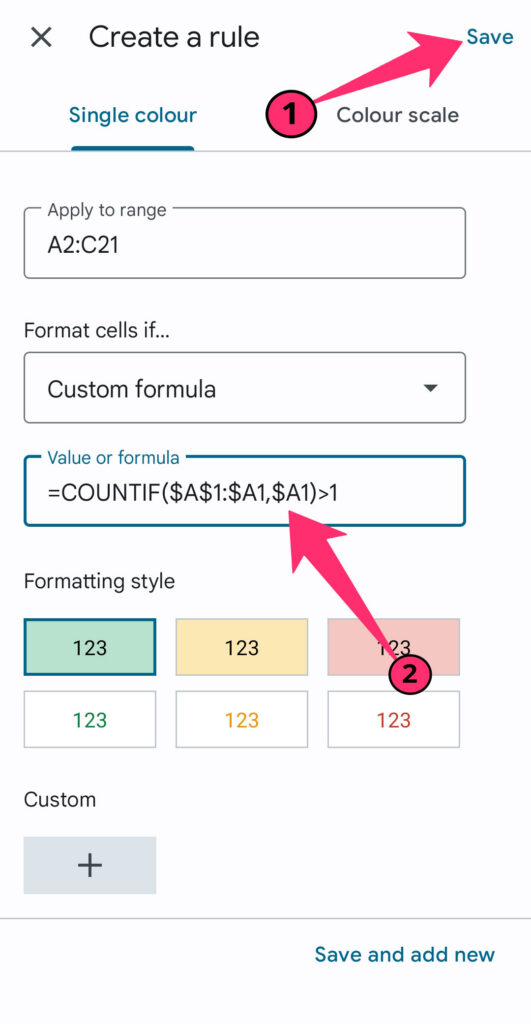
• Step 6: To highlight both columns and rows, enter the “=COUNTIF($A$1:$A1,$A1)>1” formula.
• Step 7: Tap on the “Done” button.

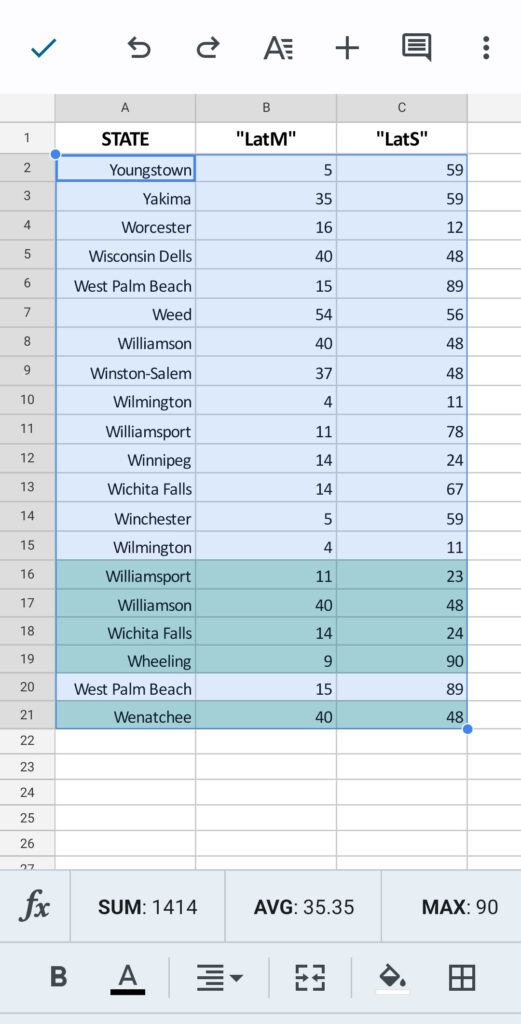
• Step 8: It will automatically highlight the cells containing duplicate values. You can then manually delete those.

Note: Once you format your Google Sheet on your app, you may need to download it on your desktop later to have a bigger view. So, check out our step-by-step guide for saving and downloading Google Sheets on your desktop.

Some Questions You May Have

Final Note

If you are working with a low to limited data range and want to remove all the duplicates, it is better to use the “Data validation” feature to remove those. However, if you need more customizations, such as deleting duplicates from a specific column, using the “Query” function or the pivot table is better.

You can also use different add-ons and plugins, such as Ablebits if you don’t have enough expertise or need to perform more complex operations.