Struggling to figure out how the time operations work in Google Sheets? I have you covered!
Time operations can be used to calculate the time difference between two events or to add or subtract a specific amount from a given time value. They can also be used in conjunction with other time-related functions, such as HOUR, MINUTE, and SECOND.
In this article, I will teach you how to use time calculations in Google Sheets. I will also provide quick and easy answers to your questions about working with them (which surprisingly do not always rely on the TIME formula).
Ready? Let’s go.
- TIME() Formula Explained
- How to Count Elapsed Time in Google Sheets
- How to Calculate Time Duration in Google Sheets
- How to Calculate Hours Between Two Time Values in Google Sheets
- How to Change Displayed Time to 24-hour Time Format (Military Time Format)
- How to Convert Hours to Minutes in Google Sheets
- Some Questions You May Still Have
- My Final Thoughts
TIME() Formula Explained
The TIME function in Google Sheets creates a time value from a given set of hours, minutes, and seconds. This function can be used to perform various time-related calculations in your Google Sheets, which we will cover in the next chapters.
Here’s the syntax for the TIME function: =TIME(hour, minute, second)
Where:
- ‘hour’ is the number of hours,
- ‘minute’ is the number of minutes,
- And ‘second’ is the number of seconds.
For example, if you want to calculate the time 5 hours, 35 minutes, and 25 seconds after midnight, you can use the following formula:
=TIME(5, 35, 15)
This will return a value of 05:35:15, which is the time you’re looking for.
Now that you know how to use it and what the best use cases are, let’s think when it’s best NOT to use the TIME formula (so you have a full perspective)
When not to use the TIME function:
The TIME function should not be used to perform calculations with time values that span across multiple days. For such calculations, the DATE function should be used instead.
Also, if you’re working with time values that are already in a valid time format, you don’t need to use the TIME function to convert them.
Now it’s high time to jump on a few real-life examples
How to Count Elapsed Time in Google Sheets
You can use the following TIME function to count a time difference between two given days.
To count the difference between the time of two days, you can use the following TIME function.
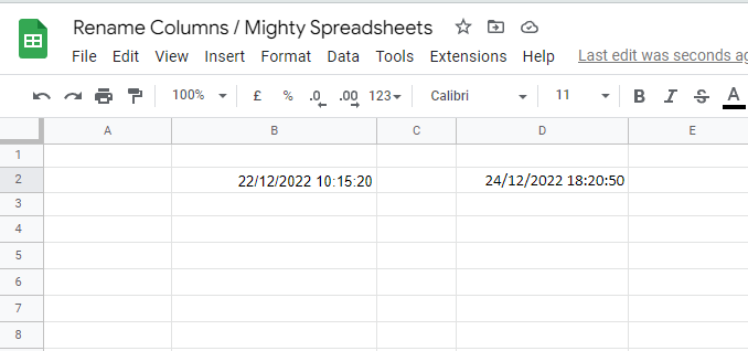
Step 1: Decide the dates you want to calculate the time difference and ensure both dates have the time mentioned.
Step 2: Enter the formula =TEXT(B2-D2-INT(B2-D2),"HH:MM: SS") and replace the cell number with the one you want to use the formula for.
I have selected the cells as shown in the image attached below. The cells have dates and times in the HH:MM:SS format.
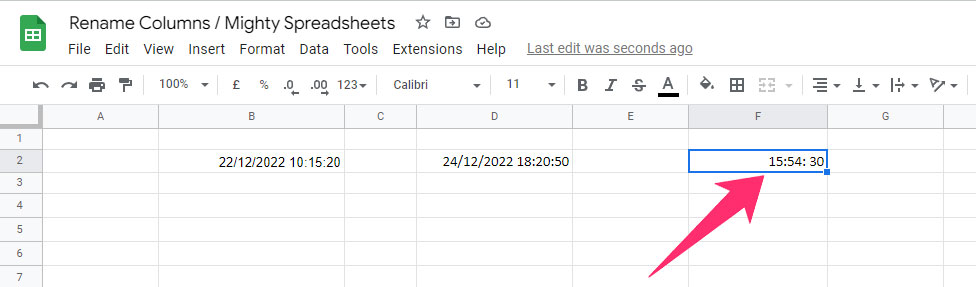
Step 3: After using the formula, the function automatically subtracts the elapsed time to show you the difference.
This is the result after using the formula:
How to Calculate Time Duration in Google Sheets
Calculating time duration in Google Sheets is easy when using the TIME function. You can find the difference between the two-time values.
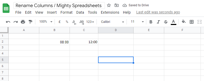
Step 1: Focus on an empty cell, enter the following formula: =B2-C2, and press Enter.
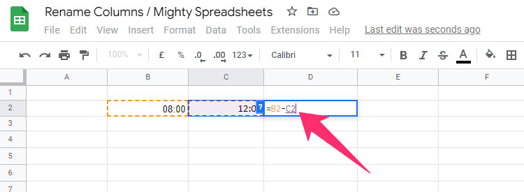
Step 2: You’ll get the answer in the selected cell.
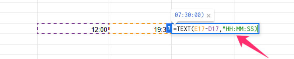
How to Calculate Hours Between Two Time Values in Google Sheets
To calculate the number of hours between two time values in Google Sheets, you need to use simple arithmetic.
Here are the steps to follow:
Step 1: Enter the start time in cell A1, then enter the finish time in cell B1
Step 2: In a third cell (say C1), use the TEXT function, subtract the start time from the finish time, and provide the format (in our case HH:MM:SS , which stands for Hours, Minutes, and Seconds)
Step 3: The operation above will return “5:30”, which is the time difference. If you are interested in hours only, you can change the format to “H”
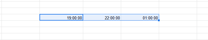
How to Change Displayed Time to 24-hour Time Format (Military Time Format)
Using the military time format makes the data look more presentable. Plus, it eliminates confusion. You can easily change the time value from AM/PM format to 24-hour format with a few clicks.
Step 1: Select the time values you want to change the format for.
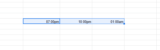
Step 2: Click on Format, select Number, and click on Time (HH:MM:SS).
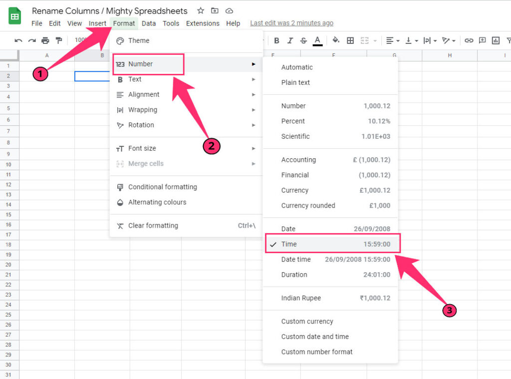
Step 3: The format of selected time values will be changed to the military format.
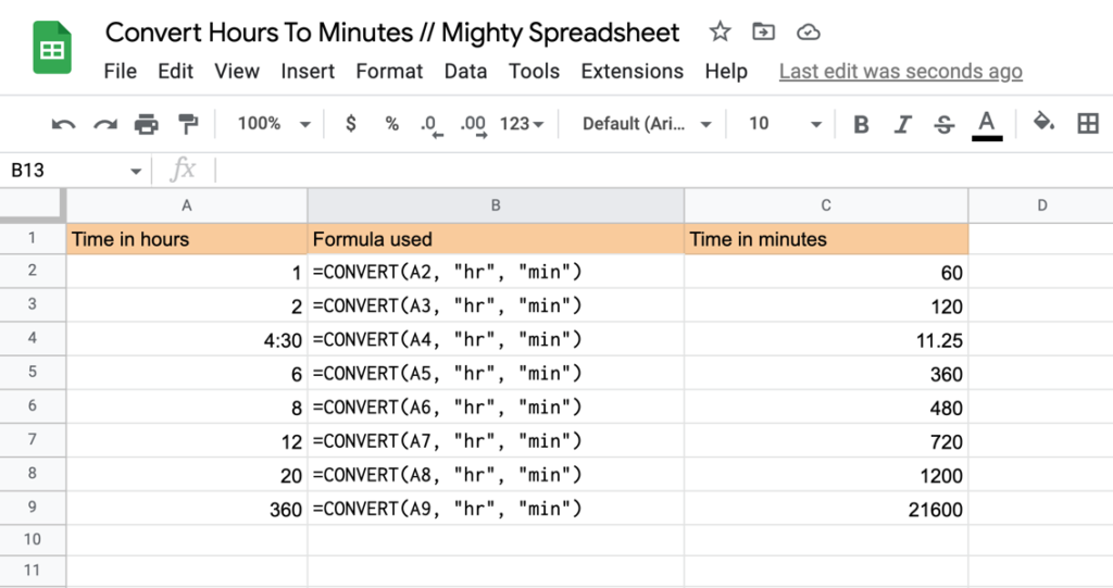
How to Convert Hours to Minutes in Google Sheets
To convert hours to minutes, you can use a CONVERT formula. The CONVERT formula converts various units of measurement, including time.
The syntax for the convert formula is as follows: CONVERT(value, start_unit, end_unit)
Step 1: Enter the number of hours you want to convert into a cell. For example, you can enter the number of hours in cell A1.
Step 2: In another cell, enter the following formula: =CONVERT(A1,"hr","min") and press Enter to apply it.
Step 3: That’s it. You should now see the number of minutes that fits the number of hours you put inside the A cell.
Some Questions You May Still Have
Is there a TIME function in Google Sheets?
Yes, there’s a built-in TIME function in Google Sheets. It creates a time value from a given set of hours, minutes, and seconds. TIME function can be used to perform various time-related calculations in your worksheet.
How do I timestamp a time in Google Sheets?
You can create a static timestamp in Google sheets by pressing “Command/Control” + “:” This keyboard shortcut will insert the current date and time into the cell.
What is the easiest way to calculate the time difference?
The easiest way to calculate the difference between two time values is to subtract the start time from the end time just like so: A2-B2
My Final Thoughts
As you can see, you have many options if you want to perform time calculations in Google Sheets. The simplest one is as easy as using the TIME function, but you can actually add, subtract and convert time in any way you want.
I hope this article made it easier for you to digest and understand, but if you still have any questions, please ask them in the comments.