How to Use Date Functions in Google Sheets (Add, Change, Format Dates Like a PRO)

Posted on February 13, 2023February 13, 2023 by Luke

This article aims to be a detailed guide on how to use date functions in Google Sheets.

Since there are many date functions, remembering them can be daunting, so I’ve made a short list of some functions you’ll find helpful. Read on to learn these functions and how to use them in Google Sheets.

Tips: Bookmark this article so you don’t miss out on these important formulas.

Essential Date Formulas in Google Sheets

Below, I have curated a list of some important date functions to use in Google Sheets. Also, I’ll show you how to use these formulas, with pictures attached.

If you need a brief comparison, you can use the table below.

If you want to see the formulas in action, you can copy this spreadsheet, where I prepared a few examples for you.

Function	Syntax	Definition
TODAY	`TODAY()`	Enters today’s date
NOW	`NOW()`	Enters today’s date and time
YEAR	`YEAR(date)`	Extracts year from a provided date
MONTH	`MONTH(date)`	Extracts month from a given date
DAY	`DAY(date)`	Extracts day from a given date
DAYS360	`DAYS360(start_date, end_date, [method])`	Calculates the number of days between two dates
DATEIF	`DATEIF(start_date, end_date, unit)`	Calculates the number of days, months, or years between two dates
YEARFRAC	`YEARFRAC(start_date, end_date, [day_count])`	Returns the number of years (including fractional ones) between given dates (using specified day count convention)
EDATE	`EDATE(start_date, months)`	Returns a date that is before or after a specified amount of months from the given date
EOMONTH	`EOMONTH(start_date, months)`	This function returns a date that represents the last day of a month. The month is a specified number of months before or after another date.
WEEKDAY	`WEEKDAY(date, [type])`	This function returns a number representing the day of the week for the given date.
WEEKNUM	`WEEKNUM(date, [type])`	The function returns a number that shows which week of the year the given date is in.
WORKDAY	`WORKDAY(start_date,end_date, [holidays])`	Returns the date after a specified number of working days.
NETWORKDAYS	NETWORKDAY(start_date,end_date, [holidays])	Calculates the number of net working dates between given dates

The table containing essential DATE related formulas

TODAY: Display the Current Date

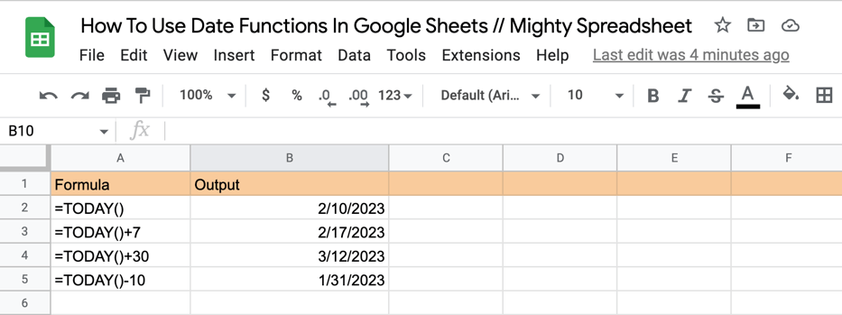
To enter the current date into the spreadsheet, you can enter =TODAY() in the cell where you want the result to appear. The function shows you the current date as per your location.

It’s important to remember that the TODAY() formula value will be updated every time you update your worksheet

You can combine the TODAY() formula with other mathematical operations. For example, you can use it like so:

=TODAY()+7 to calculate the exact date in one week’s time
=TODAY()+365 to calculate the date in one year
=TODAY()-180 , to calculate the exact date that was 180 days ago

NOW: Display the Current Date and Time

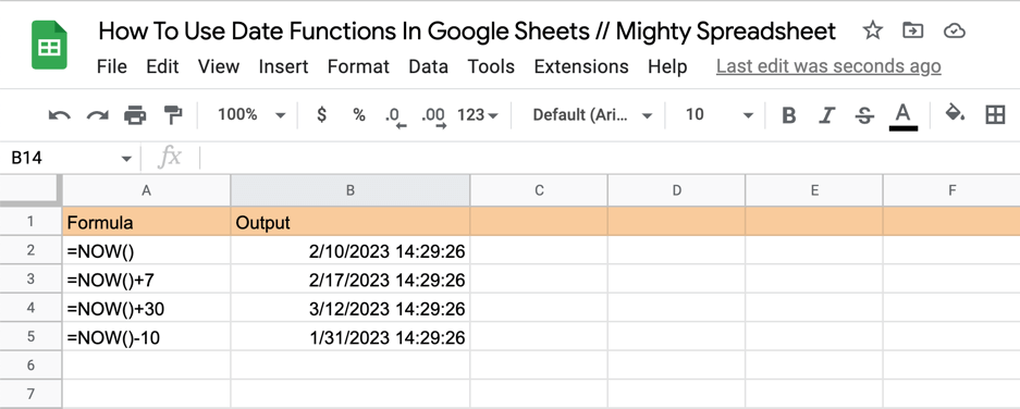
You can use =NOW()function to get the current date and time. The function returns two values, including the date and time. The values that you get are fetched based on your current location.

One important thing to notice is that the NOW() formula value will be recalculated each time your refresh your sheet

You can perform different types of operations using the NOW() formula.

For example, you can calculate the date that will be 7 or 30 days from now or what date was 10 days ago just like so:

=NOW() + 7
=NOW() + 30
=NOW() - 10

YEAR()

In Google Sheets, the YEAR() function can be used to extract the year from a provided date value. The formula for using the YEAR() function is as follows: =YEAR(date) and always returns the year in 4 digits format.

The YEAR formula can be used in combination with other formulas or perform a mathematical operation on them. For example:

YEAR(NOW()) will return the current year
YEAR(A2)-YEAR(B2) will return the difference in years between two given dates

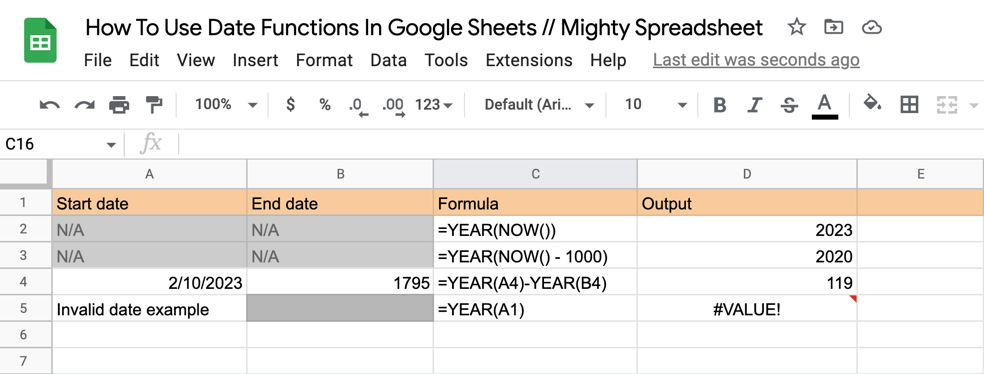
Note: The YEAR() function only works with valid date values. The function will return an error if the cell reference or value you provide is not a valid date.

MONTH()

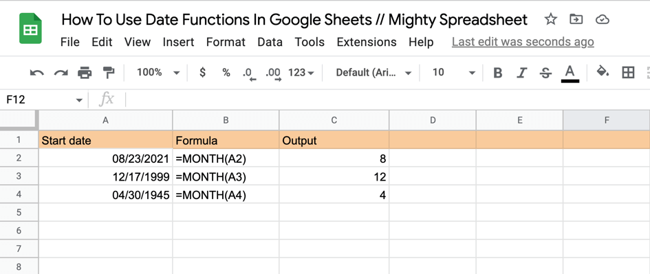
The MONTH() function in Google Sheets can be used to extract the month from a date value in a cell. The syntax for using this function is as follows: =MONTH(date)

If a cell contains the text string 8/23/2021 or a formula that returns a date value in the form 8/23/2021, this would also return 8 as a result when you use the Month() function.

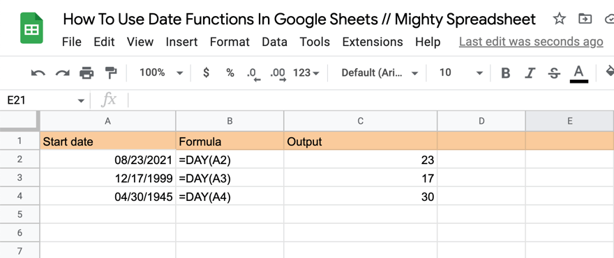
DAY()

You can use the DAY() function just like the YEAR() and MONTH() functions to get the day of the month in a Google spreadsheet. The DAY() function returns the day as specified on the particular date.

For example, if the selected date is 8/23/2021, the function will return “23” as the output.

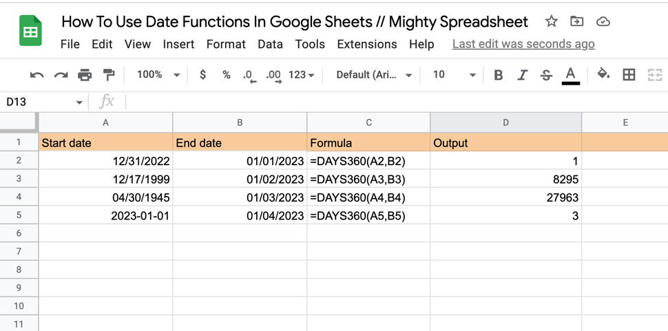
DAYS360()

You can use this date function to calculate the number of days between two dates based on a 360-day year.

The syntax for using the DAYS360() function is DAYS360(start_date, end_date, [method])

The default value for the method is 0, which stands for the “US method.” All other values provided to the method argument will represent the “European method.”

You can read about the nitty-gritty details here, but the main takeaway is that the function always counts 30 days as one month, even if the actual number of days in a month is different.

Let’s jump to a few examples:

The difference between the last day of the 2022 year and the first day of 2023 will be one day
The difference between the 17th of December 1999 and the 2nd of January 2023 will be 8295 days, and so on

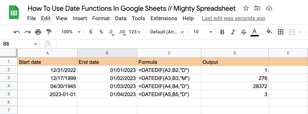
DATEDIF()

This particular date function helps you to calculate the number of days, months, or years between two dates. The syntax for using the DATEDIF() function is as follows: =DATEDIF(start_date, end_date, unit)

Start_date and end_date are the dates for which you want to calculate the difference (it can be a number of days, months, or years).

Furthermore, “unit” helps you get the output in the format you want. Here are some examples you can use as a unit argument:

“Y” – the number of whole years between given dates
“M” – the number of whole months between given dates
“D” – the number of whole days between given dates
“MD” – the number of days between given dates after subtracting whole months.
“YM” – the number of whole months given dates after subtracting whole years.
“YD” – the number of days between given dates, assuming they were no more than one year apart.

One thing to note here is that the DATEDIF() function only works with valid date values. The function will return an error if the cell references or values you provide are not valid dates.

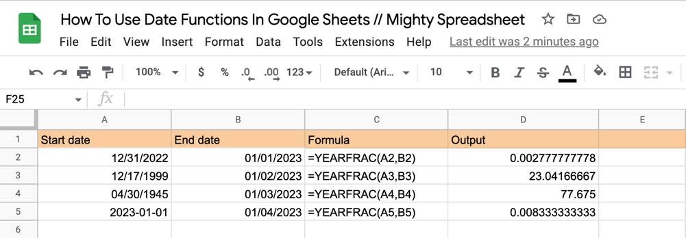
YEARFRAC()

Using the YEARFRAC() function, you can easily calculate the fraction of a year between two dates. The syntax of this formula is: =YEARFRAC(start_date, end_date, [date_count_convention])

This function is especially useful when doing any financial-related operations, like figuring out how much of the year has gone by or how many years are between two different dates.

The [date_count_convention] argument is an indicator of which day count method to use. The default is 0, which uses NASD 30/360 method (assuming 360 days a year, 30 days a month).

If you want to use the YEARFRAC() function for non-finance-related purposes, then I would recommend setting the value to 1, which assumes the actual number of days between dates.

Let’s have a look at some examples in the screenshot below. You will notice that the output is very often quite detailed, so you may consider rounding the numbers up to fit your specific purposes.

EDATE()

Using the EDATE() function, you can calculate the date that is a specified number of months before or after a start date. The formula for using the EDATE() function is: =EDATE(start_date, months)

Here the start_date is the starting date, and months is the number of months before or after the start date that you want to calculate.

For example, to calculate the date that is 3 months after January 1st, 2023, you can use the following formula:

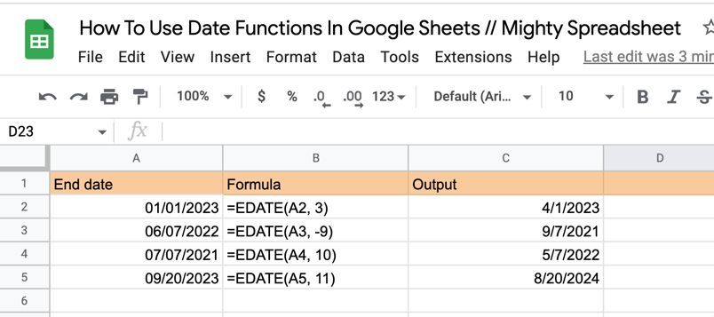
If you change it to a negative number, it will give you the date in the past.

EOMONTH()

This date function works exactly like the EDATE() function, but it calculates the number of months between a start date and an end date. The formula for using EOMONTH() is: =EOMONTH(start_date, end_date)

For example, to calculate the number of months between December 31, 2022, and March 31, 2023, you can use the following formula: =EOMONTH("2022-12-31", "2023-03-31")

The formula will return “3” as a result.

WEEKDAY()

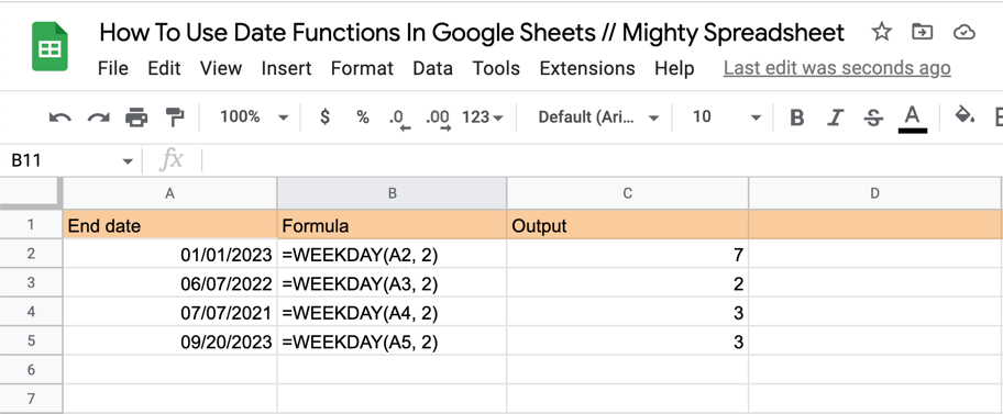
The WEEKDAY() function can be used to determine the day of the week for a given date.

The syntax for using the WEEKDAY() function is as follows: WEEKDAY(date, [type])

The “date” is the date you want to determine the day of the week for. For example, to determine the day of the week for December 31, 2022, using the default numbering system, you can use the following formula as shown in the image.
The “type” specifies which day of the week should be used as the first day of the week:
- 1 (default) – Sunday is the first day of the week
- 2 – Monday is the first day of the week
- 3 – Monday is the first day of the week (but it’s counted as 0, not 1)

What’s worth mentioning is that the formula returns the day of the week in a numeric form, so if you’d like a text output, you need to play with number formatting.

WEEKNUM()

Using the WEEKNUM(), you can determine the week number for a given date.

The syntax for using the WEEKNUM() function is as follows: =WEEKNUM(date, [type])

Where:

“date” is the date you want to determine the week number for. For example, to determine the week number for December 31, 2022, using the default numbering system, you can use the formula: =WEEKNUM("2022-12-31")
The “type” specifies which day of the week should be used as the first day of the week (works the same way as it does for the WEEKDAY function)

WORKDAY()

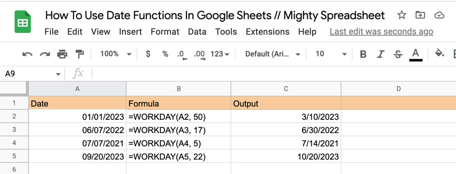
With the WORKDAY() function, you can easily calculate the date that is a specified number of workdays before or after a start date.

The syntax for the WORKDAY function is as follows: =WORKDAY(start_date, days, [holidays])

Where:

start_date – is the date from which you start counting
days – is the number of working dates from the date given (if negative, then counts backward)
holidays – optional holidays to consider

For example, to calculate the date that is 3 workdays after December 31, 2022, you can use the following formula:

=WORKDAY(“2022-12-31”, 3)

NETWORKDAYS()

If you want to calculate the number of workdays between two dates, you can use “NETWORKDAYS().” The syntax for using this date function is: =NETWORKDAYS(start_date, end_date, [holidays])

The start_date and end_date are the dates between which you want to calculate the number of workdays. “Holidays” is an optional argument that specifies a range of cells containing dates considered holidays that should be excluded from the calculation.

For example, to calculate the number of workdays between December 31, 2022, and January 4, 2023, you can use the following formula: =NETWORKDAYS(“2022-12-31”, “2023-01-04”)

This returns 3 as the output since January 1 and 2, 2023, are holidays and are excluded from the calculation.

How to Change Date Format in Google Sheets

You can use two methods to format time in Google Sheets, and below I have explained both.

How to Format Time in Google Sheets

If you want to change the time in military format, you can do it within a few clicks. Here are the steps you can follow:

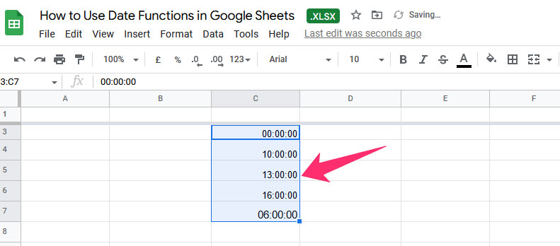
Step 1: Select the time values you want to change the format for.

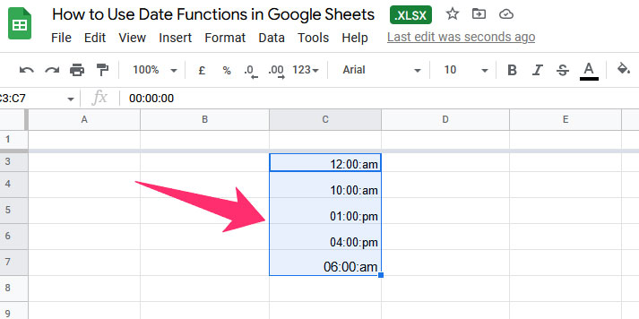
Step 2: Click on Format from the Menu Bar, select Numbers, and click on Time.

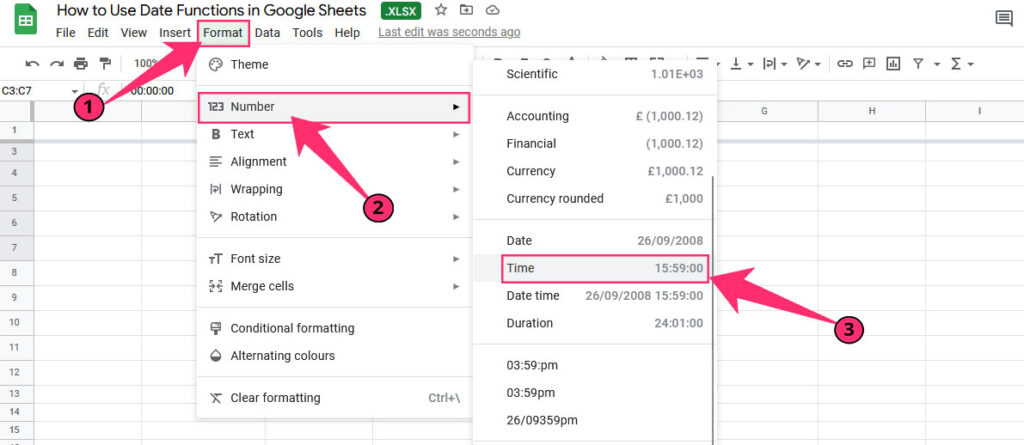
Step 3: The time values will be formatted as you want.

How to Change Date Format in Google Sheets to DD/MM/YYYY

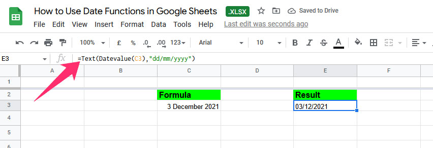
You can combine two functions to change the date format in Google Sheets. These functions are “Datevalue()”, and “Text()”. Here’s an example of how to use these functions:

Select the cell or cells that contain the dates you want to change.
In the formula bar, enter the following formula: =TEXT(DATEVALUE(A1), "dd/mm/yyyy")
Press Enter to apply the formula. The date in the cell will be changed to the specified format.
Here’s the result after using this formula.

How to Calculate Dates in Google Sheets

You can use multiple methods to add or subtract dates in Google Sheets. Let’s have a look at the most common and easy methods you can use.

How to Add Dates in Google Sheets

You can use the + operator or the DATE() function to add dates in Google Sheets.

Here’s an example of how you can use the + operator to add days to date:

Step 1: Select the cell where you want to display the result.

Step 2: In the formula bar, enter a formula like the following: =Cell Number+ Number of days you want to add.

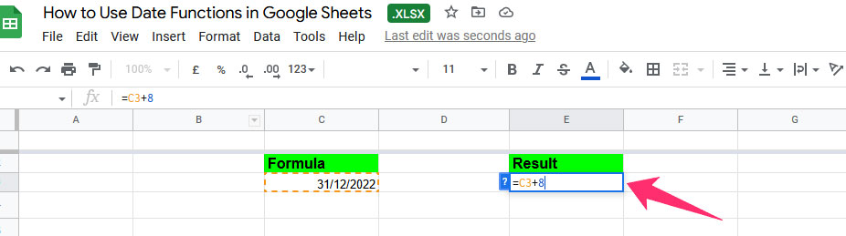
Step 3: Press Enter to apply the formula. The result will be the date in cell C3 plus 8 days.

Step 4: In this example, the cell number contains a date value, and the + operator is used to add 8 days to the date.

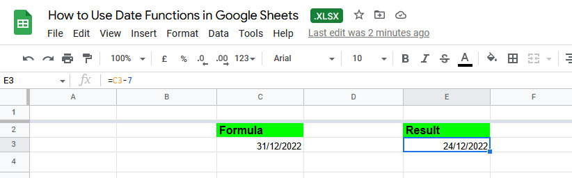
How to Subtract Dates in Google Sheets

Subtracting days from a date also works like adding days.

Step 1: Select the cell where you want to get the output, and enter the Cell number – the number of days you want to subtract.

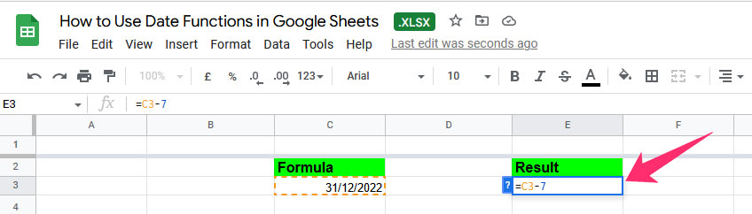
Step 2: Press Enter, and 8 days will be subtracted from the selected date.

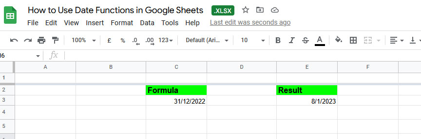
How to Calculate Current Date + 7 Days

Step 1: Select the cell where you want the result, and enter: =Today() + Number of days you want to add. You can use a “-“, if you want to subtract days from the current date.

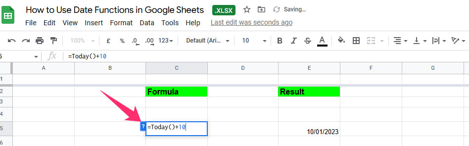
Step 2: Since the date at the time of writing this article is “31/12/2022”, after adding 10 days to it, the result comes as “10/01/2023”.

Real-Life Examples and Struggles

Here are some real-life examples of date functions in Google Sheets and the struggles you might experience. Read on to learn how you can overcome them.

How to Sort and Filter Dates in Google Sheets

To sort and filter dates in Google Sheets, you can use the sorting and filtering options in the toolbar or the SORT() and FILTER() functions in a formula.

Here’s how to sort dates using the toolbar:

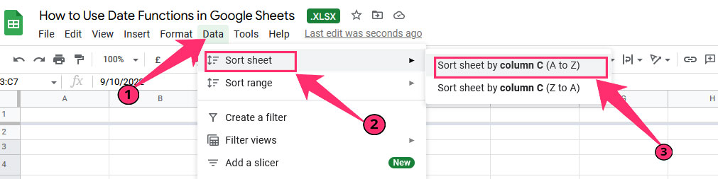
Step 1: Select the range of cells that contains the dates you want to sort.

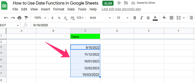
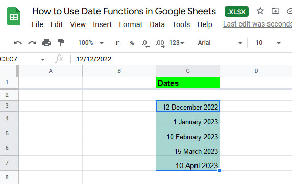
Step 2: Click the “Data” menu, then click “Sort sheet by column A-Z” or “Sort sheet by column Z-A” to sort the dates in ascending or descending order, respectively.

How to Organize Due Dates in Google Sheets

There are several ways you can organize due dates in Google Sheets:

Use a column for the due dates, and sort the sheet by that column to view the tasks in order of the due date.
Use conditional formatting to highlight tasks that are overdue or due soon. To do this, select the range of cells containing the due dates, click the “Format” menu, select “Conditional formatting,” and set up rules to highlight cells based on their date values.
Use the FILTER() function to create a separate sheet that only shows tasks that are overdue or due soon. For example, you can use a formula like =FILTER(A1:B10, A1:A10<TODAY(), A1:A10>=TODAY()-7) to show tasks that are overdue or due within the next 7 days.

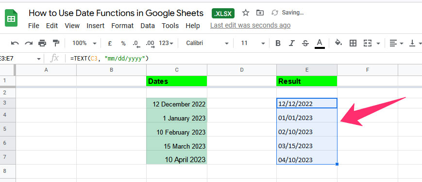
How to Change Date to String in Google Sheets

To change a date to a string (text) value in Google Sheets, you can use the TEXT() function. The syntax for using the TEXT() function is as follows: TEXT(value, format).

The “value” is the date value you want to convert to text. The “format” is a text string specifying the format you want to use.

Here’s an example of how you can use the TEXT() function to change a date to a string:

Select the cell or cells where you want to display the result.

Select the cell for change date to string

In the formula bar, enter a formula like the following: =TEXT(Cell number, "mm/dd/yyyy")

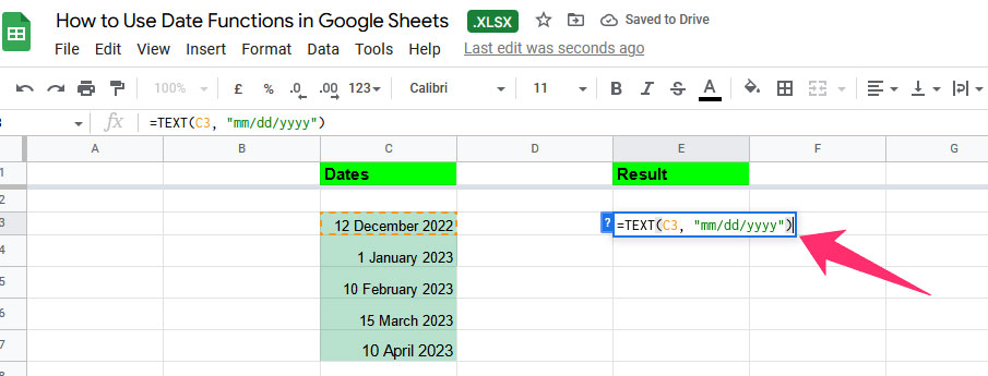
Press Enter to apply the formula. The date in the cell number will be converted to a string in the specified format.

How to Show Current Year in Google Sheets

You can use two functions to show the current year in Google Sheets. These functions include Year() and Today().

Here’s an example of how you can use these functions to show the current year:

Select the cell where you want to display the result.
In the formula bar, enter the following formula: =YEAR(TODAY())
Press Enter to apply the formula. The result will be the current year.

In this example, the TODAY() function returns the current date, and the YEAR() function extracts the year value from the date.

Note that the TODAY() function will update automatically to reflect the current date, so the result of the formula will always show the current year.

You can also use the YEAR() function to extract the year value from a specific date by replacing TODAY() with the cell reference or date value you want to use. For example, =YEAR(A1) will return the year value of the date in the cell number.

Final Thoughts

I hope these date functions have helped you add, subtract, and format dates in Google Sheets. Make sure to change the cell number when you copy the formulas from this article to ensure you don’t get an error.

Got any questions regarding date functions? Let me know by commenting down below.

Stay tuned with us for more informative posts, and become a pro at using Google Sheets.