There are two ways to filter the data in Google Sheets. You can filter the data only for yourself, or you can filter it in a way that will affect other people who have access to the sheet.
I will cover both cases deeply in this guide.
How to Filter Data in Google Sheets without Affecting Other Users (with Filter Views)
Imagine that 20 people have access to a spreadsheet. Everyone has a different task and needs to do custom filtering to finish their job.
If each person started messing around with this spreadsheet and changed data for others, it would be challenging to use it.
Fortunately, that’s where the “Filter Views” feature comes in.
It’s one of my favorite features in Google Sheets for a few reasons:
- It allows you temporarily remove unnecessary data leaving only what’s needed for a given scenario
- It doesn’t affect others’ works
- It will enable you to save the view for future reference
- It allows you to create multiple views and jump between them
- It will allow you to share your filter view with other users
I will cover those points in more detail, but let’s start with the basics first.
How to create Filter Views in Google Sheets
To create Filter views, you need to follow these steps:
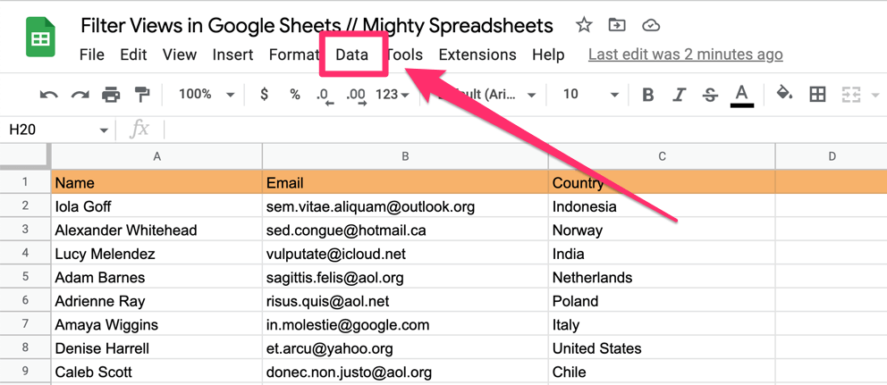
Step 1: Click on “Data” in the Options Menu
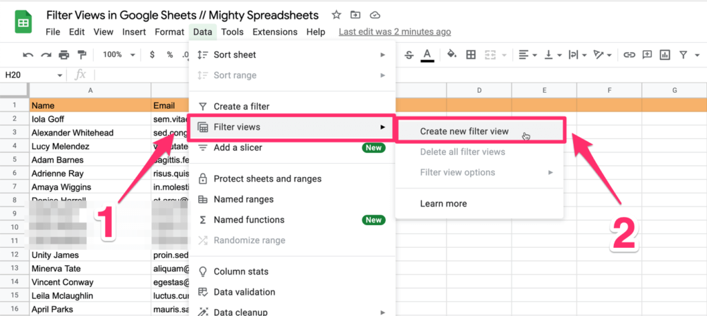
Step 2: Now, hover over “Filter views” and select “Create new filter view”
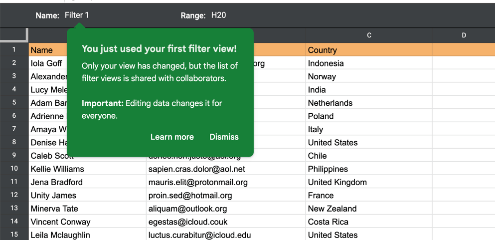
Step 3: You will notice that your spreadsheet looks slightly different now. That’s because you entered a filter views mode.
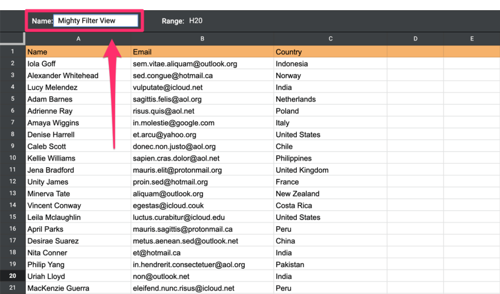
Step 4 (Optional): You can quickly name your filter view to reference it whenever you want.
Step 5: You will also notice that the first rows of your sheet act like headers, with filter icons on the right-hand side. Click on the filter wherever you need it and start playing with the data.
PRO-TIP: With a more extensive set of data, I usually lock the first row so it shows the header names at all times without the need to scroll up to alter the filters.
Now let’s go through different filtering options that you can go through after clicking on the filter icon.
3 Ways To Filter Data in Google Sheets
Here I gathered some helpful information about possible filtering options.
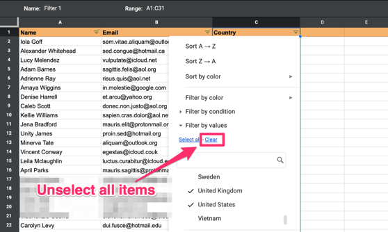
Filter Data by Values in Google Sheets
Sorting by values is perhaps the simplest thing you can do here.
Step 1 (Optional): That’s only my preference, but very often, I start by unselecting all the items
Step 2: Select all options that match your criteria
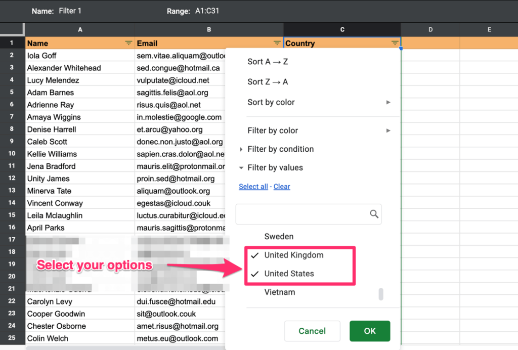
You can also use the search bar if the list is quite long.
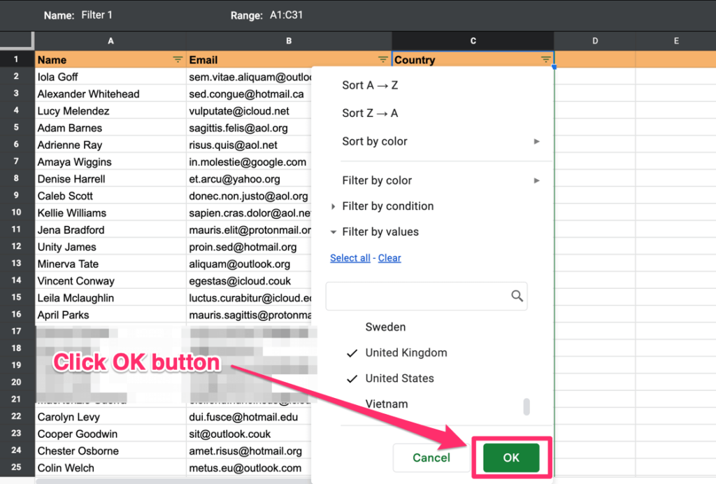
Step 3: Click the OK button and enjoy your filtered list of items.
Note: Columns with a filter applied have a very different icon from those without. I find this tip helpful, especially when working on someone else’s data.
If the filtered list is not enough for your task. You can also sort the remaining items in 3 ways:
- Sort A to Z
- Sort Z to A
- Sort remaining items by color
By the way, I’ve written more detailed guides on sorting entries in ABC order and sorting entries by color, so make sure you check these articles too.
Filter Data by Color in Google Sheets
Using colors is a great way to visually group data by specific criteria. Very often, you fill some cells with green background or turn the text red not to miss it when you browse the data next time.
The exciting thing is that you can filter out elements using the colors they have.
Do you want only yellow cells visible? Easy!
Do you want only green text present? Checked!
Here’s how to do it:
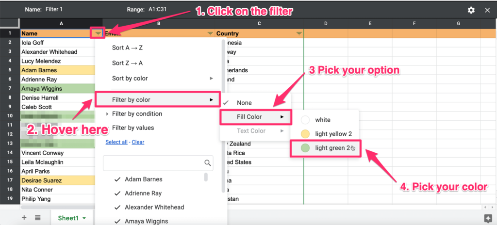
Step 1: Hover over the “filter by color” option and pick the action you want to take:
- Fill color if you’re going to filter by background color
- Text color if you wish to filter text by its color
- None is an excellent option for removing the existing filters
Step 2: Pick a color from the list.
Remember that this option will only be accessible if you have a minimum of one additional color on your spreadsheet. (The default for the background is white, and the text defaults to black.)
By the way – Did you know that you can also sort items by color? Read this article to learn how filter in Google Sheets by Color
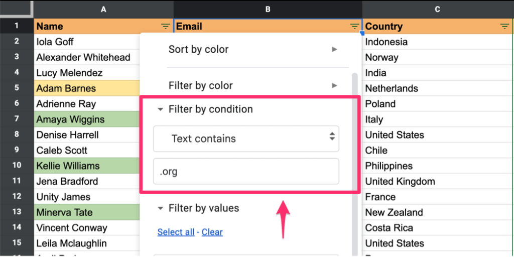
Filter Data by Condition in Google Sheets
I left it for the end because it’s the most powerful way of filtering your data, allowing you to create advanced rules for filtering.
You can:
- Filter by cell text value (i.e., if it contains a string of text, starts or ends with certain characters, etc.)
- Filter by date
- Filter by cell’s number value (is greater than X, lesser than Y, between some values, etc.)
- Write a custom formula.
All you need to do is to select the option that is good for you and fill it with the value.
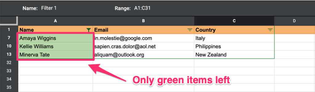
For example, let’s assume that you want only to see entries that use the “.org” email address.
Here’s how you can set your filter:
How To Share Filter Views with Other Users
Ok, you are filtering the data without affecting it for other people, but there’s a chance that you will want to share your filtered view with someone.
It’s effortless to do this:
Step 1: Select the filtered view you want to share and ensure it’s active (go to Data > Filter Views and select one of the filters that you created)
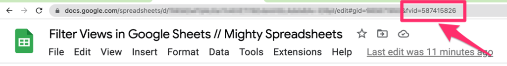
Step 2: Copy the URL from your browser
Step 3: Share it with whoever you’d like.
Note: You will notice that the (quite long) URL will contain the “fvid” (which stands for “filtered view ID”) parameter that looks more or less like this "&fvid=1293552164"
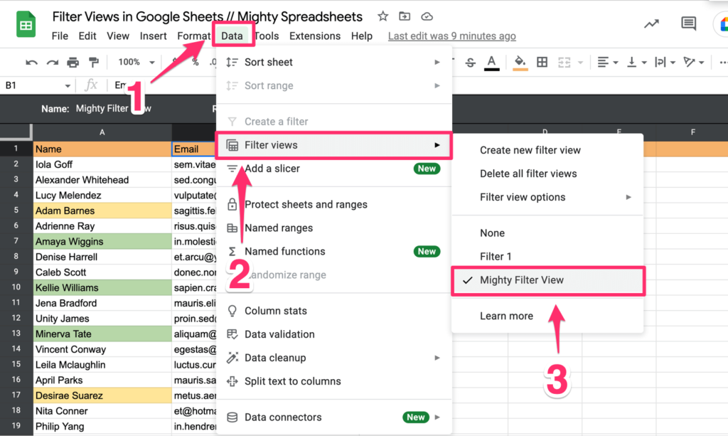
How To Switch Between Filter Views in Google Sheets
Every time you create a Filter View, it is remembered by Google Sheets.
You can easily refer to any filtered view you’ve created by simply going to Data > Filtered views and selecting the one you need from the list.
That’s the easiest way to toggle between the views you created.
Note: Although you can create unlimited filtered views, only one can be active at once.
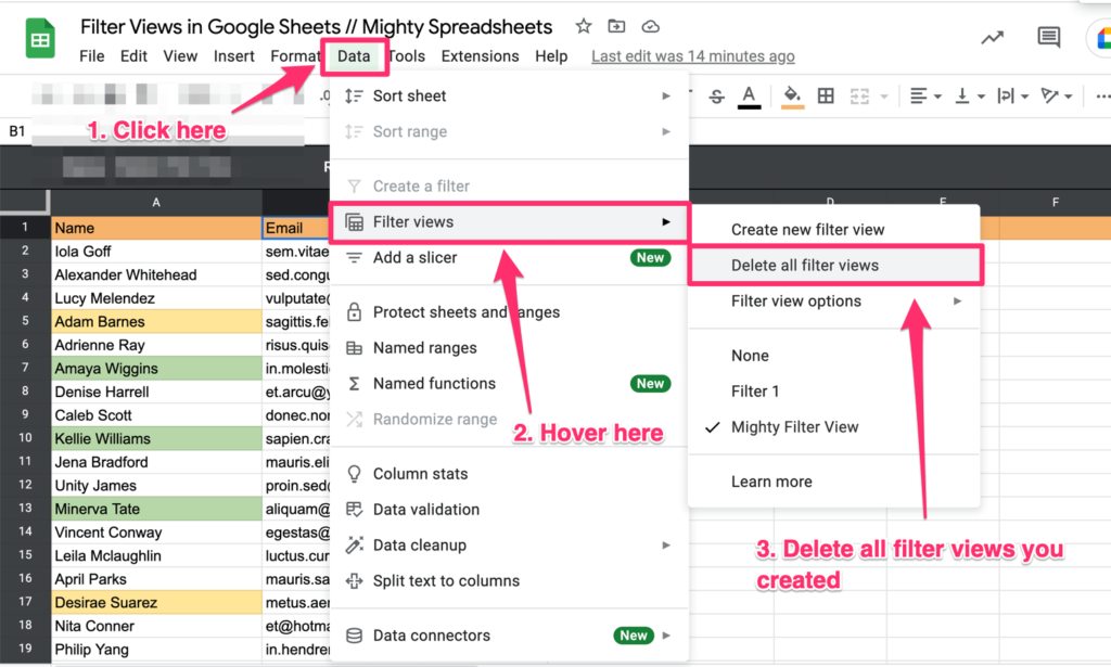
How to Remove Filter Views
You have two options to remove the filter views:
- Remove all filter views at once
- Remove a particular filter view that you don’t longer need.
To remove all filter views you’ve created, go to Data > Filter Views and click on the “Delete Filter Views” option.
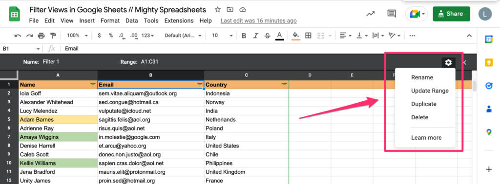
To remove a particular view without altering the other ones that you have, you need to follow these steps:
Step 1: Go to Data > Filter Views and select the view you want to be removed.
Step 2: Click the cog icon on the right side of the document and select the “Delete” option.
How To Filter Data for Everyone
As you already know, you can filter data without making any changes to the spreadsheet for other users. But let’s also cover a different approach – one where filters are applied universally so that all collaborators can see the changes.
The interface, process, and filtering/sorting options remain the same as when you created a “filter view.” The only difference is that you initiate it in a different place.
Here’s how the whole process looks like (without the nitty-gritty details that we covered in the previous section)
Step 1: Select the area you want to apply the filters to
Step 2: in the Options Menu, go to “Data” > “Create filter.”
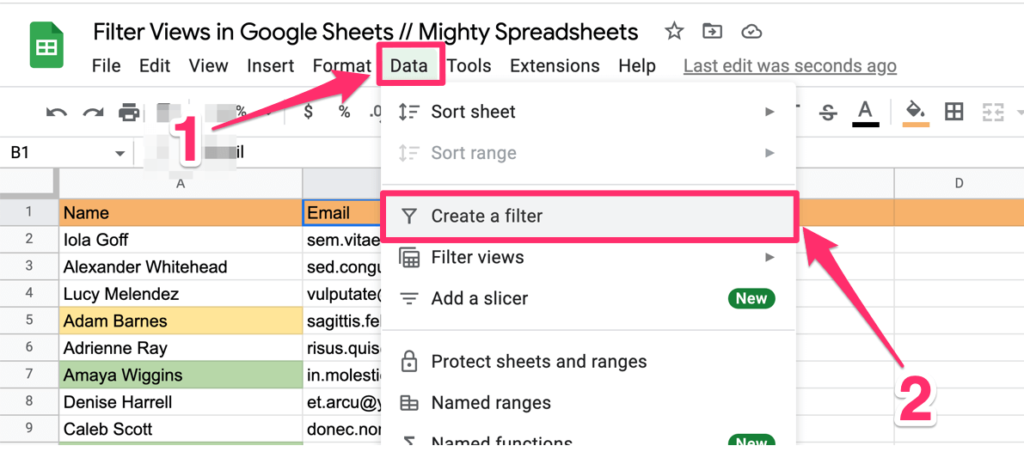
Step 3: Click on the filter icon and set the filters as you like
You have the same options here. You can filter by:
- color
- values
- condition
And if, after the whole operation, you’d like to remove the filters, all you need to do is navigate to “Data” > “Remove filter.” in the Options Menu.
How To Filter Multiple Columns in Google Sheets
Although filtering by applying only 1 criterion is relatively easy, you may struggle with using filters for two, three, or multiple columns at once.
The steps you will need to take depend on the type of filter you’d like to apply.
If we are speaking of multiple filters, there are two options you may want to consider:
- AND logic (Both criteria must be completed simultaneously to deliver results.)
- OR logic (At least one of the criteria must be met to show results)
Filter Multiple Columns Using the “AND” logic
For the sake of this example, let’s use a Marvel Cinematic Universe Spreadsheet that I found on Reddit and adjusted a bit so it better matches our example (if you want to follow along, you can copy it by clicking on this link)
Setting the AND logic in Google Sheets is relatively easy. You can even do it in the UI by clicking on filter icons.
In our exercise, we will want only to see the Marvel movies that:
- Have an IMDB rating of 7.0 or higher
- AND there is an infinity stone involved in the plot
This is what you need to do:
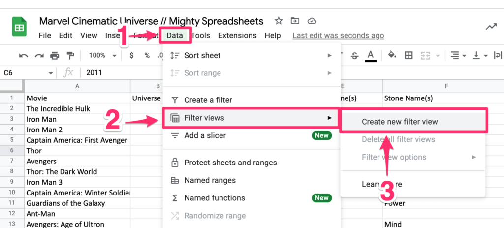
Step 1: Create a new Filter view by clicking on the Data > Filter Views > Create new filter view
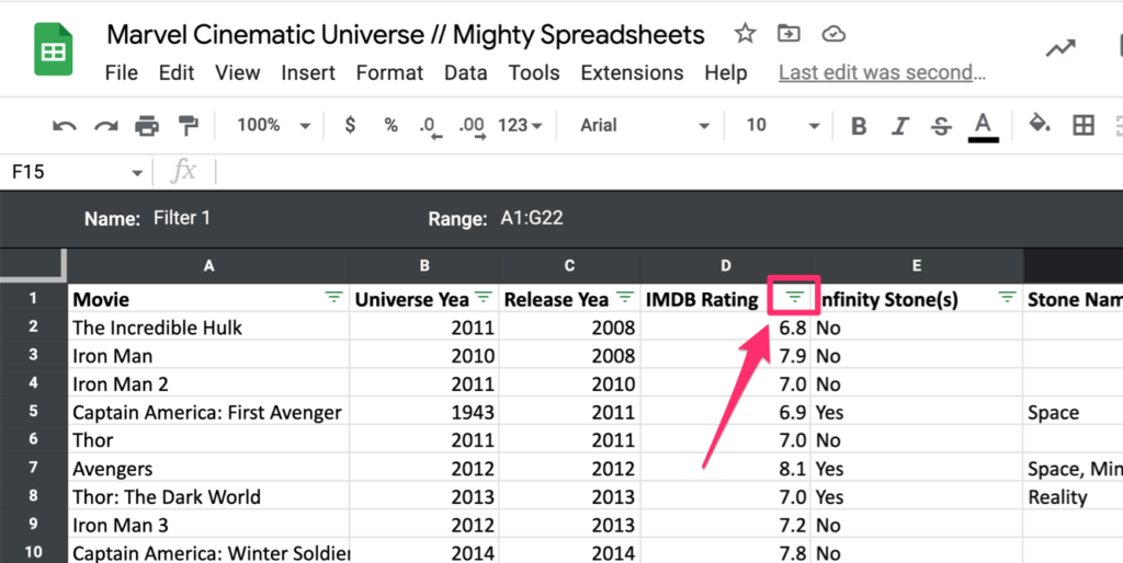
Step 2: Click on the first set of filters (IMDB ratings)
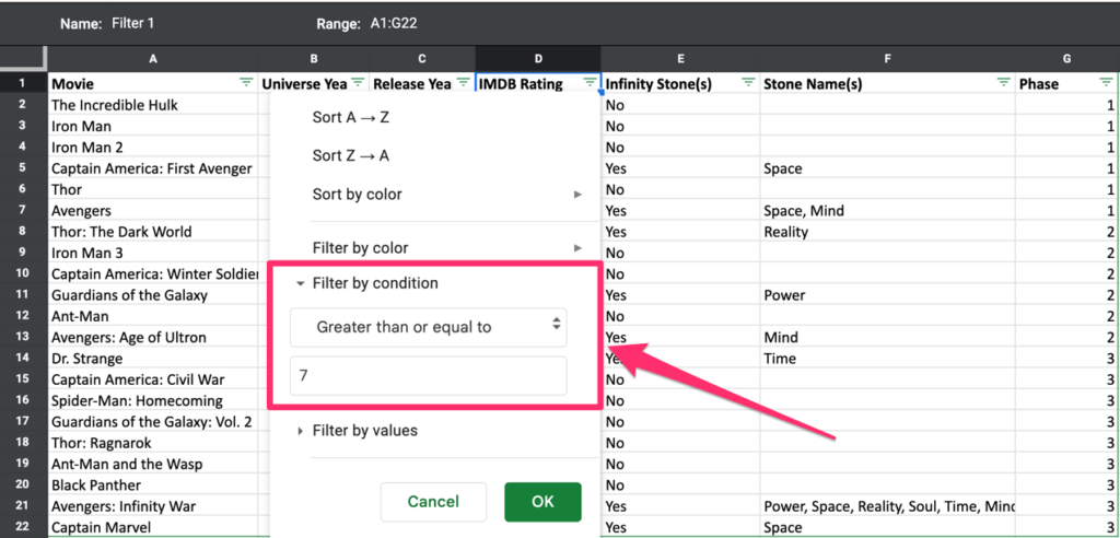
Step 3: Select the “Filter by condition” filter and pick the “greater than or equal to” option
Step 4: Type “7” in the value box and click the OK button.
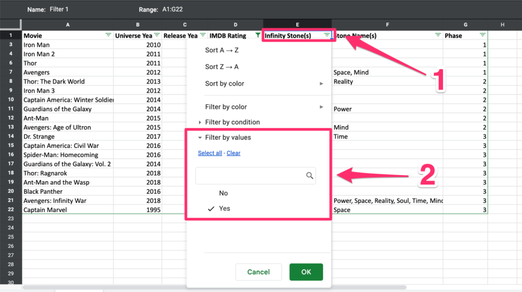
Step 5: Click on the filter icon next to the “Infinity stone” column.
Step 6: Select the “Filter by value” option and make sure that only the “Yes” option is unchecked
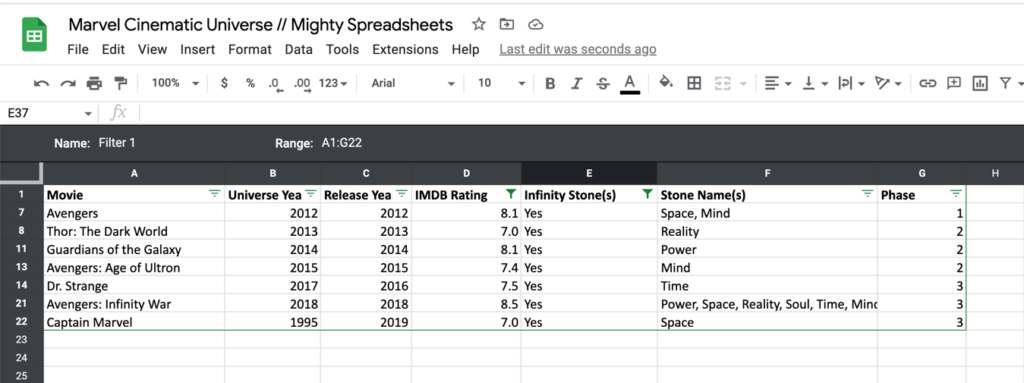
Step 7: Observe the final result
Filter Multiple Columns Using the “OR” logic
Although it may require extra effort, writing a custom formula can make this task achievable.
Let’s jump to our example and create a filter that will show titles that:
- The universe year is 2010 or before
- The actual release year is 2010 or before
Here’s what you need to do:
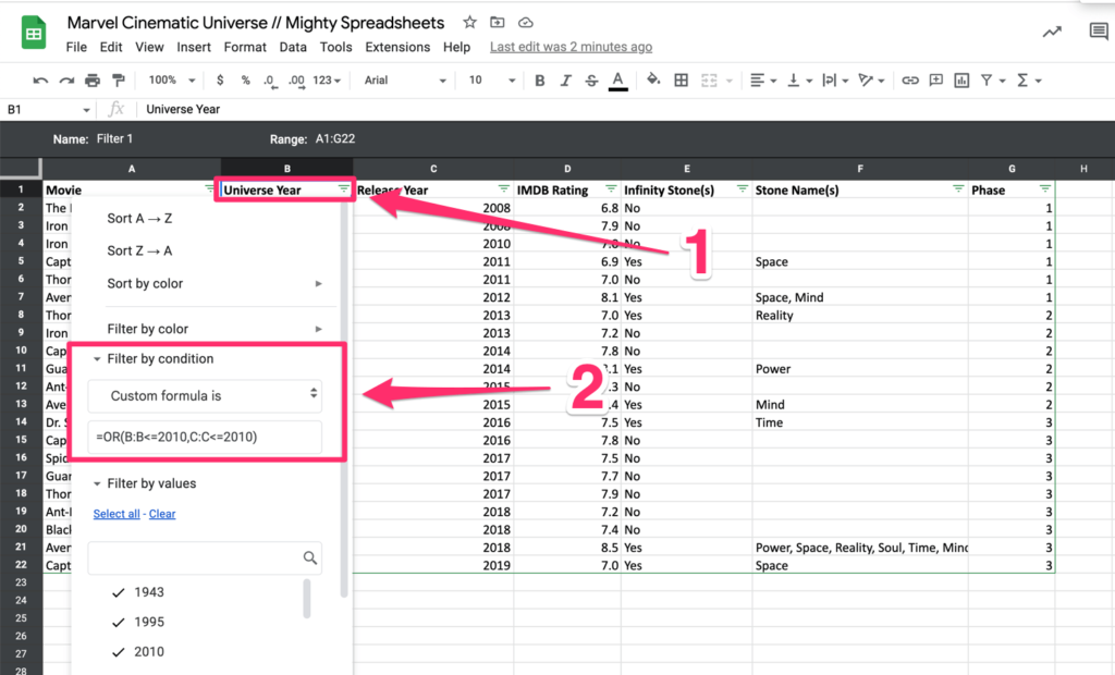
Step 1: Click on the filter icon next to the “Universe year”
Step 2: Select the “Filter by condition” filter and pick the “Custom formula is” option (the one on the very bottom)
Step 3: Write this formula: =OR(B:B<=2010,C:C<=2010) And click OK button
Here’s a breakdown of the formula we’ve used:
- OR function (returns TRUE when one of the conditions is met)
- B:B<=2010 – means all entries from the B column that value is 2010 or smaller
- C:C<=2010 means all entries from the C column that value is 2010 or smaller
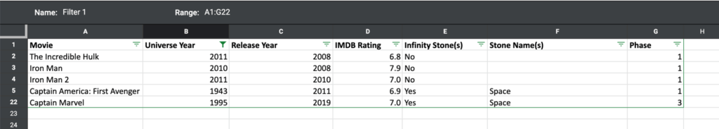
Step 4: This is the final effect you should be seeing:
Your Takeaways:
- Filtering data in Google Sheets can be a powerful way to organize and manage your information.
- There are two ways of filtering data in Google Sheets:
- First, filters the entries only for the current user
- The second one filters for everyone
- Each filter has three options. You can filter by:
- color
- values
- condition
- You can filter more than two columns simultaneously with both AND and OR logic.
Is that anything that’s missing from the article? Let me know in the comments below.