A Google Sheets header row is important and helps label and organize the data. It makes understanding and interpreting the data easy, especially when working with large data sets.
Fortunately, creating a header row in Google Sheets involves only a few simple steps.
In this post, I’ll give you a quick rundown of how to insert a header in Google Sheets and how to add time, workbook title, and page numbers to the header.
How To Make A Header Row In Google Sheets
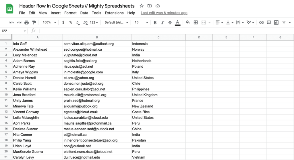
Let’s imagine that you have a Sheet filled with data like this:
First up, you need to decide where you need to make a row a header in Google Sheets.
Generally, this will be row 1 for most of us.
Step 1: On the far left, you will see the row number for each row on your Google Sheet. Right-click on the row number that should be right below the future header row
Step 2: Since you wish to create the header row right above it (for example), you can click on Insert 1 row above from the dropdown menu.
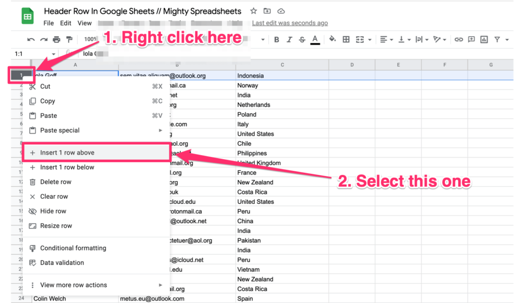
This step will create a new blank row above your sheet’s data.
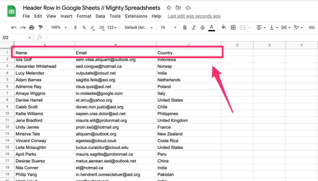
Step 3: All you need to do is to fill it with the required labels like this:
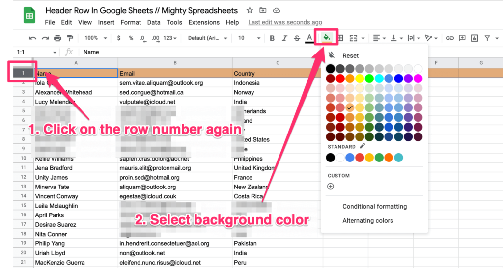
Step 4 (Optional): In the end, you can also change the background
BTW since we are speaking about background colors – check how to alternate every other row in Google Sheets
How To Make A Header Row Sticky
Making a row ‘sticky’ refers to freezing it in place. Thereafter, while scrolling down, you can see the sticky header row at all times.
- To make a sticky row header select the row by clicking on it
- Next, click on View and hover your cursor over Freeze, which will open up a drop-down menu.
- You can select the number of rows/columns you wish to freeze. Click on Up to row 1.
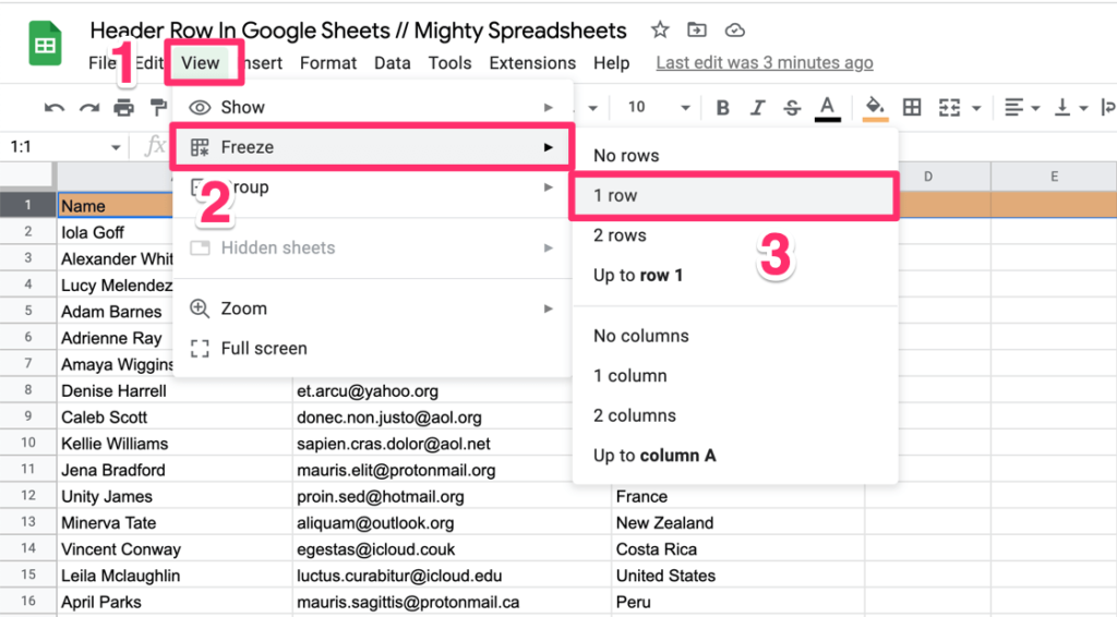
Once you select it, you can scroll through the spreadsheet while the header row remains frozen at the top.
P.S. I’ve written a more detailed guide on how to freeze a row in Google Sheets, so make sure you don’t miss it.
How To Add A Header And Title In Google Sheets For Print
There are a few options in the print menu that will take care of this.
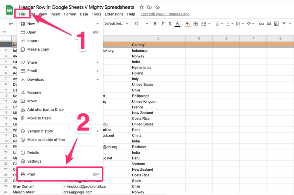
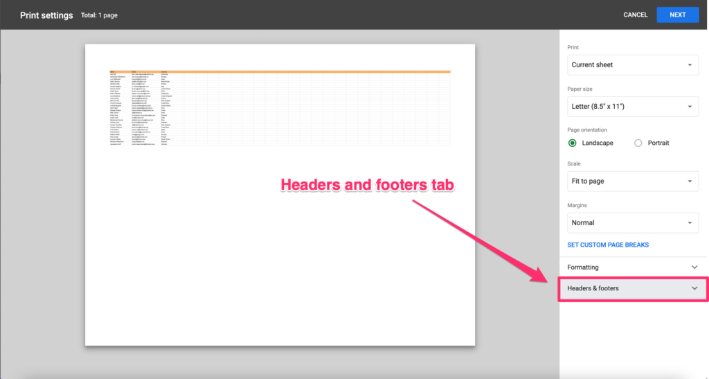
Step 1: To add a header and title, click on File from the options menu and scroll down to Print, which opens the print menu.
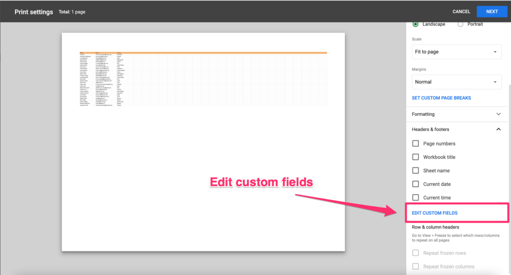
Step 2: Once you are at the print options, you will see a list of tabs. Click on Headers & Footers.

Step 3: This will open up a drop-down. Find and click the Edit Custom Fields option near the bottom of the menu.
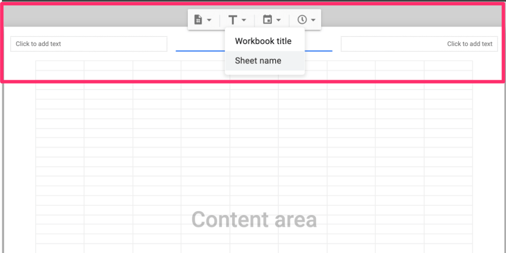
Step 4: This opens the editor, and you can now add a header and a title of your choice in any three header tabs.
How To Include The Page Number In The Header
You can add page numbers to headers using the header and footer options.
Step 1: Press CTRL + P (Windows) or Command + P (Mac) to open print options and click on Headers & Footers.
Step 2: Next, scroll down until you find Edit Custom Fields and click it.

Step 3: This will open up the header editor. Click on the section you want the page number to be on.
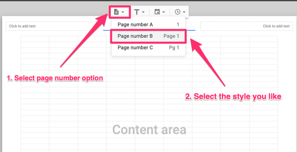
Step 4: From the small menu on top, click on the page number, which is the first option.
This will show you several styles you want the page number to be in. Select something you like, and that’s it.
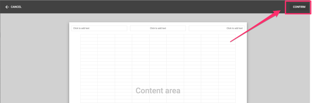
Step 5: Click the confirm button in the upper right corner and Print your sheets.
How To Include A Workbook Title In The Header
The process of adding the workbook title is pretty much the same.
Step 1: Click on File and click on Print while you’re scrolling down.
Step 2: Click on Headers & Footers next to the print options, which will show the same options.
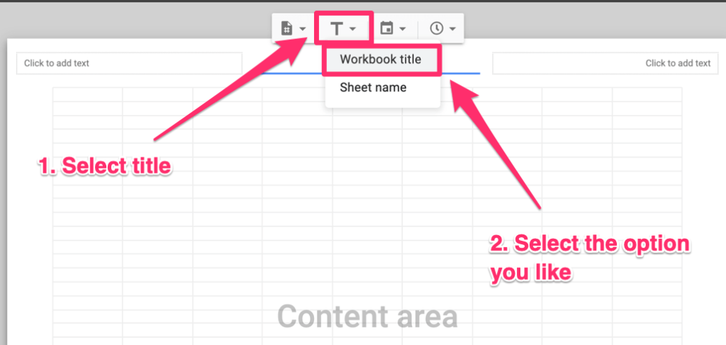
Step 3: Check the box next to the left of the Workbook title option to include the title in the Sheets header, and click Next. Make your final adjustments to the print settings (if you wish to) and click Print.
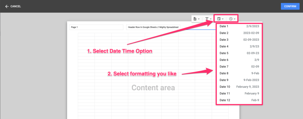
How To Include The Date And Time In The Header
Step 1: To include the date and time, Google Sheets header row, click File from the options menu, and select Print which opens up the print menu.
Step 2: This window will include a few options. Below the Headers & Footers tab, you will see tabs such as Current date and Current Time.
Step 3: Check the boxes next to these options, and Google Sheets will include the date and time in the header when printed.
Step 4: Click Next and make any final adjustments/edits to the print settings.
Step 5: And finally, click Print.
My Final Thoughts
As you can see, there are two different ways to create a header in Google Sheets. The first assumes that you want to make the first row a header in your actual worksheet, and the second one relies on the fact that you can insert a header in print mode.
You can use two simultaneously if you want your document to be easy to work with and organized when someone prints it.