Strikethrough in Google Sheets (A Complete Guide)

A Strikethrough is a great way to mark data that is no longer relevant or accurate. It’s like crossing something off your to-do list, except in your spreadsheet!

The fastest way to strikethrough in Google Sheets is to select the cell and click on the strikethrough icon on the toolbar.

In this post, I’ll give you a rundown of the different ways we can strike through in Google Sheets and how to remove and filter strikethrough formatting.

Strikethrough In Google Sheets Using The Keyboard Shortcut (Works On Mac And Windows)

The keyboard shortcut for strikethrough in Google Sheets is:

• ALT + SHIFT + 5 in you are on Windows
• Command + Shift + X if you are on Mac.

All you have to do is:

Step 1: Select the range of cells you wish to ‘strikethrough’.

Step 2: Use the keyboard shortcut that I mentioned earlier. 

This will apply a strikethrough to the text on the specific cell. However, if you only want to apply strikethrough formatting to part of the text, you need to:

Double-click the cell and highlight the part of the text you hope to strikethrough, and then press the shortcut.

PS. As you probably noticed, the text here is wrapped. Did you know there are 4 different ways to wrap a text in Google Sheets?

Do keep in mind that this shortcut works as a toggle! Therefore, if you repeat this shortcut on cells that already have strikethrough formatting applied, it will be removed.

Strikethrough In Google Sheets Using Toolbar

This option is probably the best and most convenient, as you don’t have to remember a shortcut or search for menu options.

Additionally, this is the better option if you prefer using the toolbar on your screen instead of the keyboard.

Step 1: Select the range of cells you need to strikethrough.

Step 2: Click on the strikethrough icon next to the text color icon. It’s as simple as that.

Strikethrough In Google Sheets Using The Options Menu

The third option would be to select strikethrough from the options menu.

This is probably the best option for not-so-tech-savvy users who start their adventure with Google Sheets and need to get familiar with the layout first.

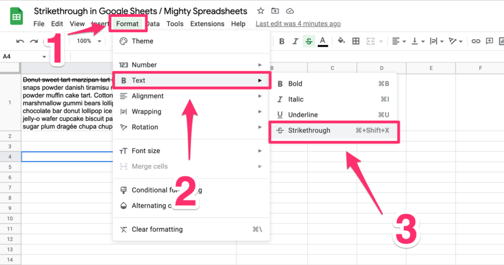
Step 1: Select the cells you want to strikethrough.

Step 2: After selecting the cells, click on ‘Format’ to view the menu. 

Step 3: Once the options appear, hover over “Text” and click on the “strikethrough” option. 

While using this method is definitely up to you, it is probably the least convenient option as it involves more steps.

How To Remove Strikethrough Formatting In Google Sheets

As we talked about earlier, the keyboard shortcut works as a toggle.

If you’ve used this shortcut, repeat it on the selected cells, and it will be removed.

Step 1: Select the cells from which you wish to remove strikethrough formatting.

Step 2: Use the keyboard shortcut again.

Similarly, the toolbar option can be used by selecting the formatted text and clicking on the strikethrough option once again. This, in turn, will reverse the action.

The same concept applies to all three strikethrough formatting options, making it simple to remove.

Step 1: Select the formatted text.

Step 2: Click on the strikethrough option in the toolbar.

Add Strikethrough Through Conditional Formatting

Conditional formatting lets you format cells in a manner that changes their appearance based on the values they contain, which is helpful.

Plus, it makes a significant difference visually as it makes things clearer and easier to identify for the reader.

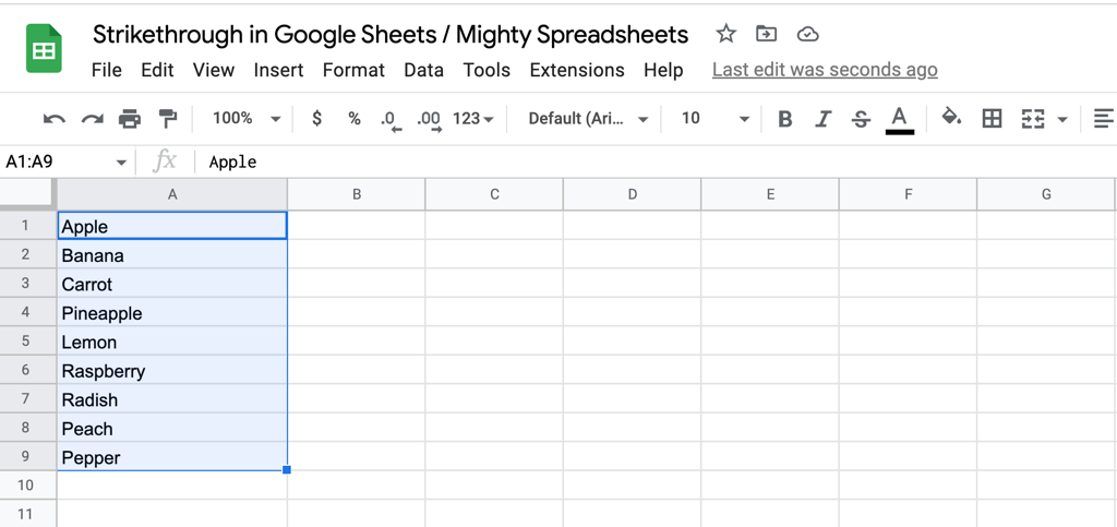
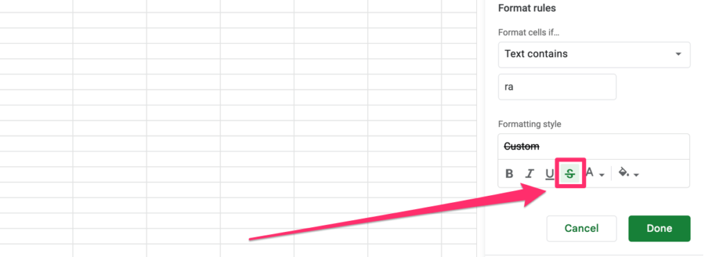
Step 1: The first step is to add a strikethrough through conditional formatting, is to highlight the range of cells you want to apply conditional formatting to. 

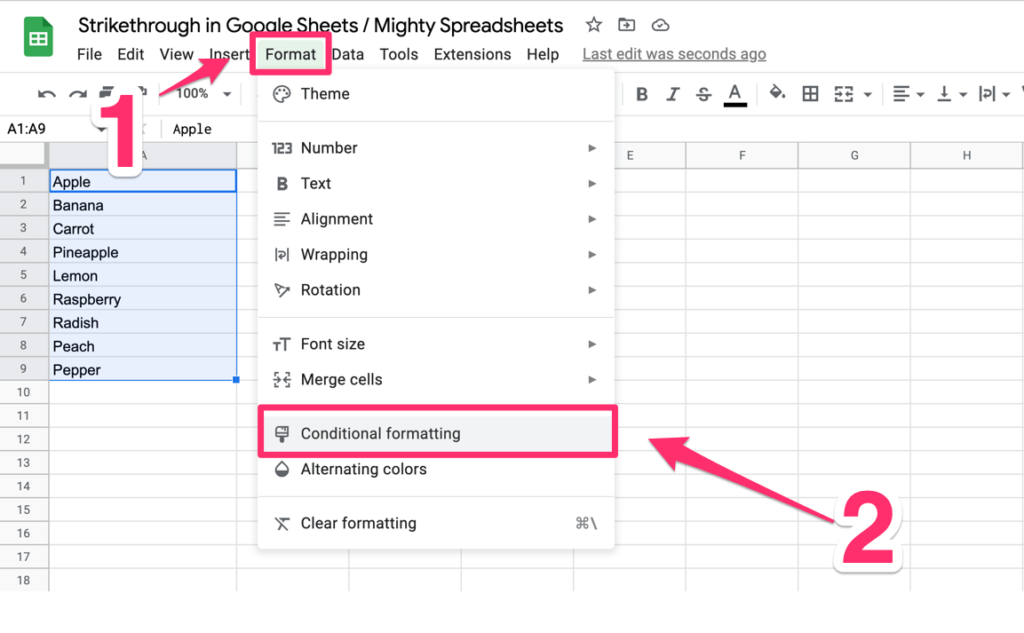
Step 2: Next, click on ‘Format’  and select ‘Conditional Formatting’. 

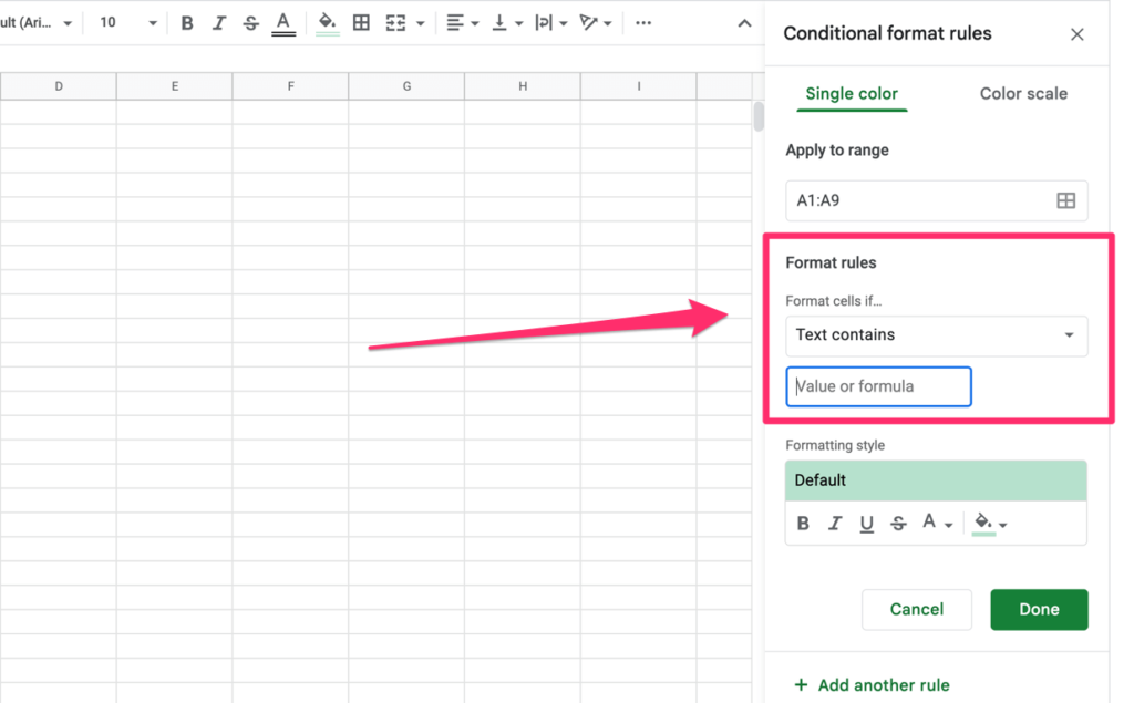
Step 3: The Conditional formatting tab section will open on the right and automatically fill in the selected range. You can use the ‘Format rules’ to set whatever rule a specific cell should have to have strikethrough styling applied. 

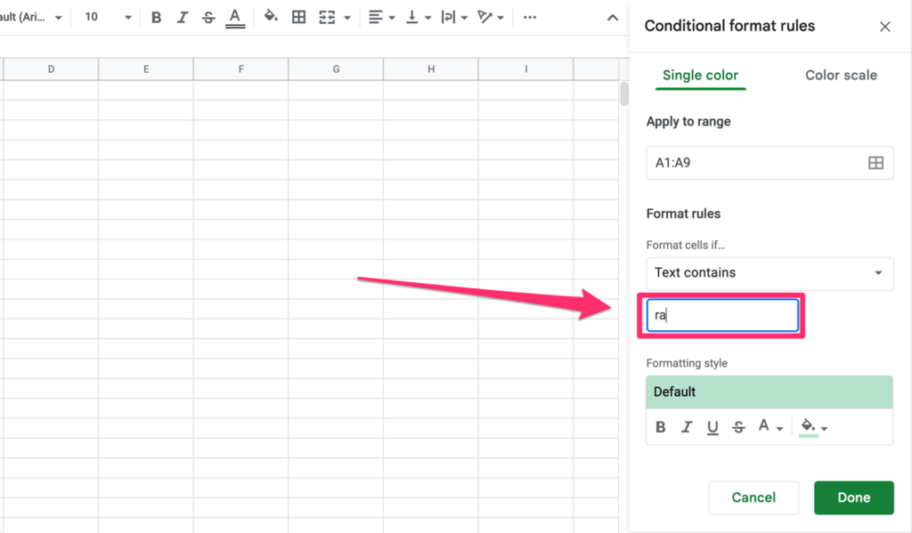
For example, if you hope to apply strikethrough to all cells in your selected range that include letters “Ra,” your format rule would “Text Contain” and the value would be “ra”

Step 4: From the formatting style, select strikethrough. And click done.

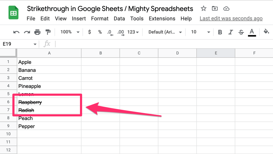
And that’s the final effect you should expect:

I created a habit tracker that uses checkboxes and strikethrough for styling. Make sure to check it out!

How To Filter Out Strikethrough Items In Google Sheets

By default, there’s no way to filter out items that have strikethrough styling applied.

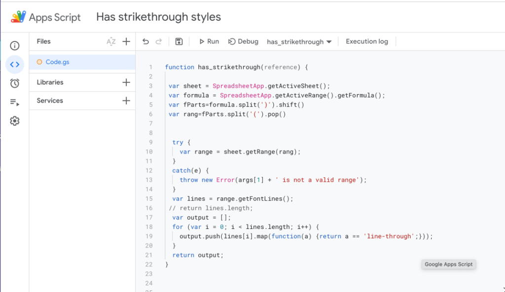
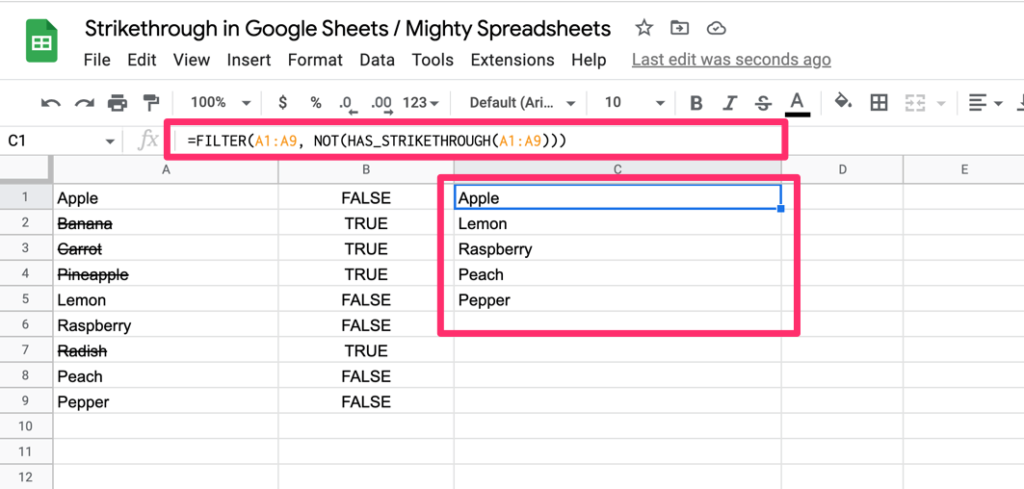
You need to create a custom function using Apps Script that checks if a cell has strikethrough styling applied (for example, you can use this snippet) and then use this function inside the FILTER function.

Your final formula should look like this: =FILTER(A1:A9,NOT(HAS_STRIKETHROUGH(A1:A9))). 

Let’s take a look a this in more detail:

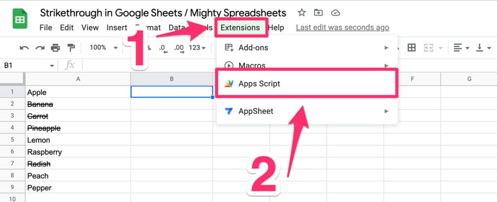
Step 1: In the Options Menu, click on Extensions > App Scripts

Step 2: Create a custom function by pasting the code linked above

Step 3: Go back to your sheet and test if the formula works

Step 4: Use our custom function inside the FILTER formula like so: =FILTER(A1:A9,NOT(HAS_STRIKETHROUGH(A1:A9)))

And here’s an explanation of what this function does:

The selected cells (A1:A9) are evaluated based on TRUE or FALSE values. Therefore, the cells that include strikethrough formatting will return TRUE, and the rest will return FALSE.

By default, The FILTER function will leave all items that return TRUE (which, in our case, are the items that have STRIKETHROUGH styles applied)

This is why we need to use the NOT function to reverse the output.

How To Count Strikethrough Cells In Google Sheets

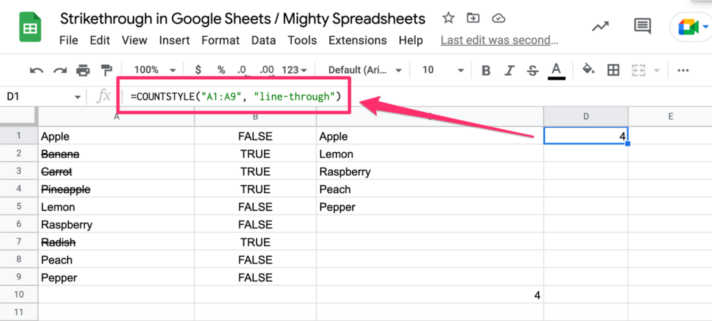
Contrary to Excel, Google Sheets don’t have an in-built function for this purpose. However, it’s possible thanks to the range of add-ons Sheets support.

In this example, I will use Custom Count and Sum, which has an excellent set of additional functions.

Step 1: Click on Add-ons > Get add-ons and search for ‘’Custom Count and Sum’’. 

This add-on has a list of functions–one of which is ‘’line-through’’. Once you have this add-on, follow the steps below.

Step 2: In order to count strikethrough cells, use the =COUNTSTYLE function

Step 3: Select the cell range and type: =COUNTSTYLE("D2:D15", "line-through")

My Final Thoughts

Strikethrough is extremely simple but, at the same time handy feature that allows changing styling of text. Although relatively limited by default, you can easily extend it with custom App Snippets code or Workspace addons and include them in your regular workflow.