This article provides a comprehensive guide on how to add alternating colors in Google Sheets.
We will cover several different scenarios that may be useful for your projects. We will also cover every possible edge case you may be facing.
This tutorial should take you about 5 minutes to complete. If you’d like to feel free to copy this accompanying spreadsheet. If you do so you will be able to follow along with the examples below.
How To Apply Alternating Colors in Google Sheets
The are a few different ways to apply alternating colors. Let’s start with the simplest one that will highlight every other row and will also cover most of your use cases.
Example 1: How To Make Every Other Row Gray in Google Sheets (Or In Any Other Color)
In this section, I will show you how to shade every other row in Google Sheets. It is a very efficient way to make your data more readable and easier to digest.
It’s also a great feature if you want to format your data as a table in Google Sheets
Here are the steps you need to follow:
Step 1 (Optional): Open the “Exercise 1 – start” worksheet
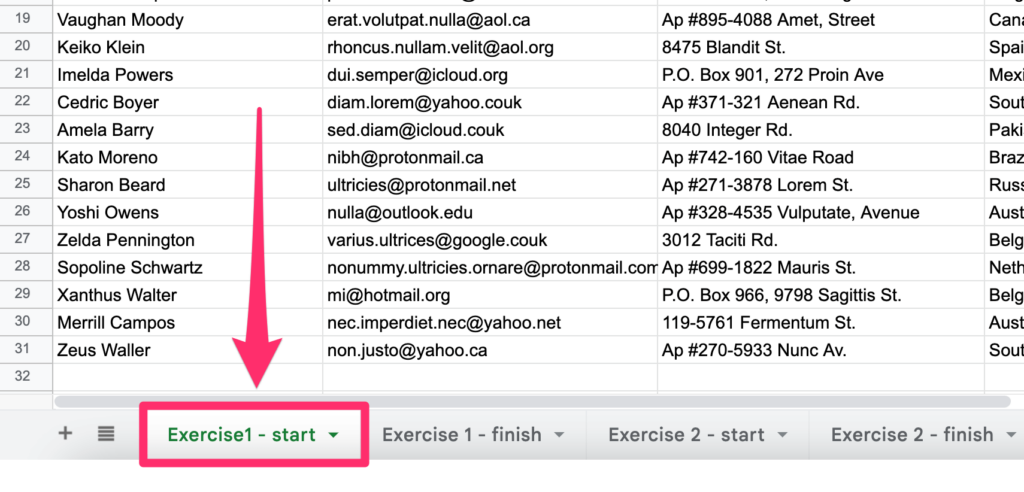
PS. If you open the exercise sheet you will notice that the first row is pinned to the top. If you are wondering how to do that feel free to check this article where I explained how to freeze cells in Google Sheets
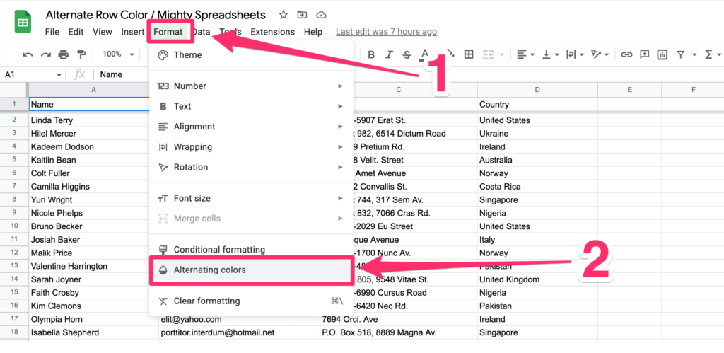
Step 2: In the Options Menu go to “Format” and select “Alternating colors”
Step 3: You will see a popup on the right-hand side of your screen.
First, select the range to be A1:D
Then you can customize the options. The default one is just going to make every other row gray.
If you have a header (like we do in the example) just make sure that you check the “header” option too.
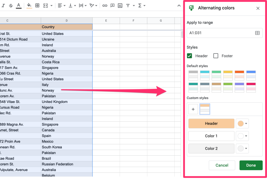
Step 4 (Optional): You can customize the colors of your layout to be whatever you’d like. You can either pick a color from the default styles or use custom ones too.
That’s how the final output should look like:
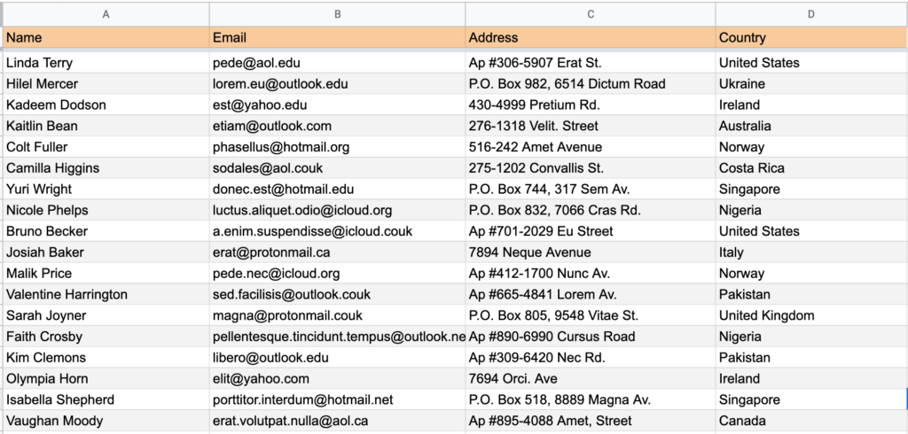
As you can see it’s super easy to do and you should be able to format your data in less than 1 minute. Plus, if you add more entries to the sheet, later on, they will automatically be formatted as well.
The only downside is that any colors that were applied before formatting will be overridden.
PS. The data is now much easier to read and follow. If you’d like to make it even better check this article where I explained how to remove gridlines in Google Sheets
Example 2: How to alternate colors every 3 or 4 rows in Google Sheets
The example mentioned above will be enough in most cases but what if you want to color every second or even the third row? That’s also possible but requires a little bit more effort.
In this exercise, we will change the background color for every third row. Here’s what you need to do:
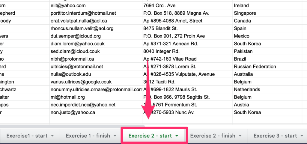
Step 1 (Optional): Open the “Exercise 2 – start” worksheet
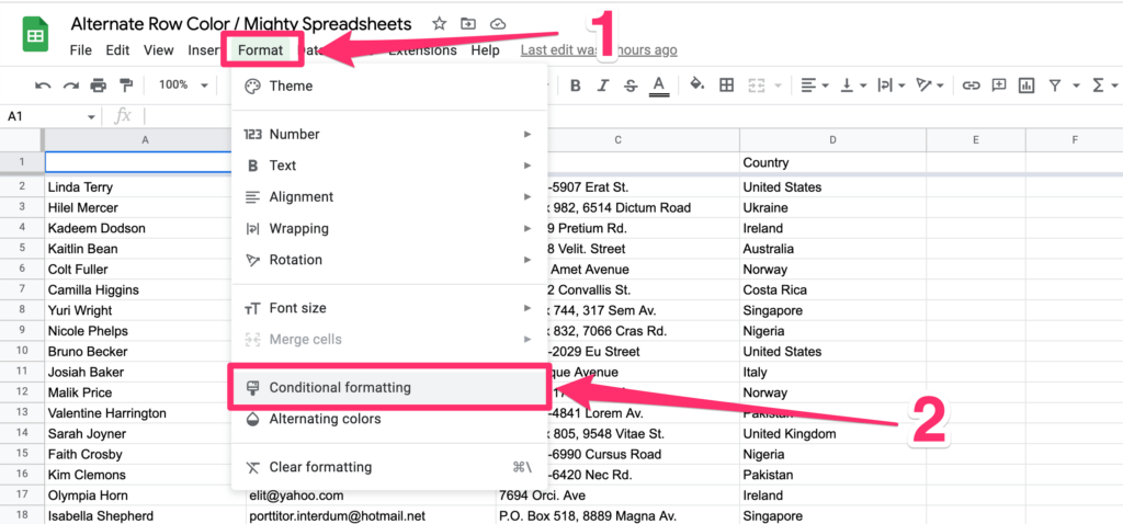
Step 2: In the Options Menu go to “Format” and select “Conditional formatting”
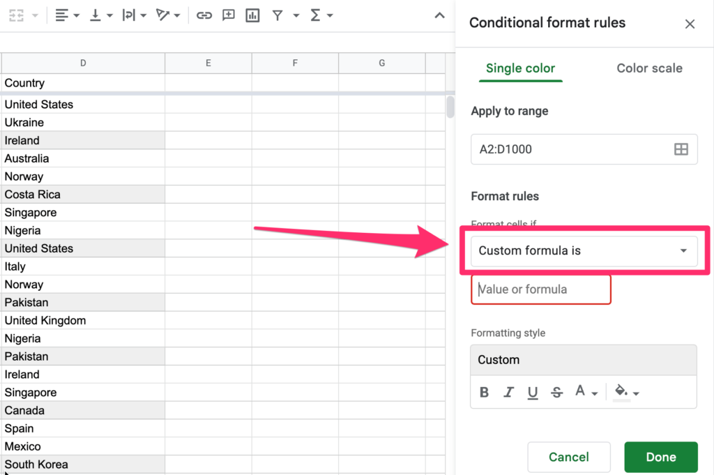
Step 3: In the pane that you will see on the right-hand side set the range to A1:D to include all rows in the sheet
Step 4: Now, find the “Format rules” section and set the “Format cells if…” to “Custom formula is”
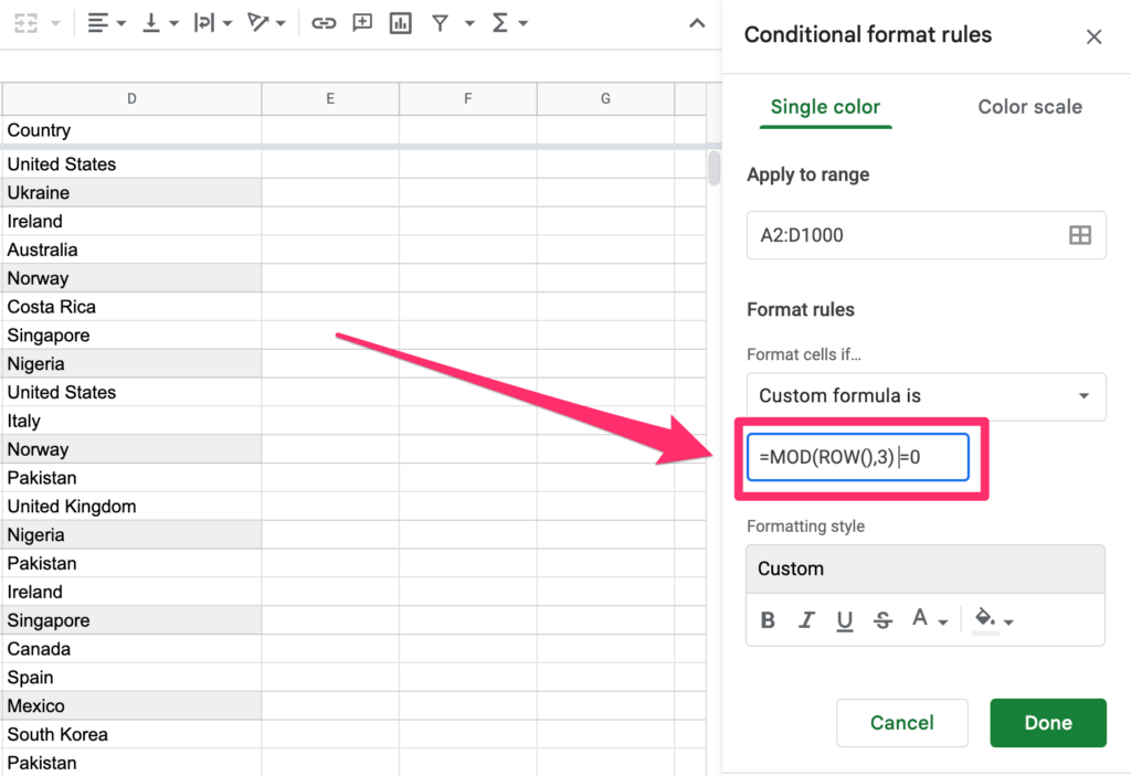
Step 5: Paste the formula into the input that will appear below: =MOD(ROW(),3)=0 and apply some formatting styles
Here’s a breakdown of the formula:
ROW()– gets the row number of each cellMOD()– Returns the result of the modulo operator (simply speaking it is what reminds us what’s left after a division operation).- The background color will only be changed when the result of the above formula returns
TRUE - So for the second row
=MOD(2,3)will return 2 which is not equal to 0 therefore the result of the function will beFALSE - And for the third row
=MOD(3,3)will return 0 which is equal to 0. That means the result of the function will beTRUEand these cells will be formatted
Step 6: Let’s optimize the formula!
As you can see the formula works perfectly well. Rows 3, 6, 9, 12 (and so on) are grey now. However, we didn’t consider the fact that we have a header in our table which we shouldn’t be considered in the calculations.
How can we fix it? It’s simple, we just need to subtract 1 (as we are offsetting the formatting by 1 row) from the general output.
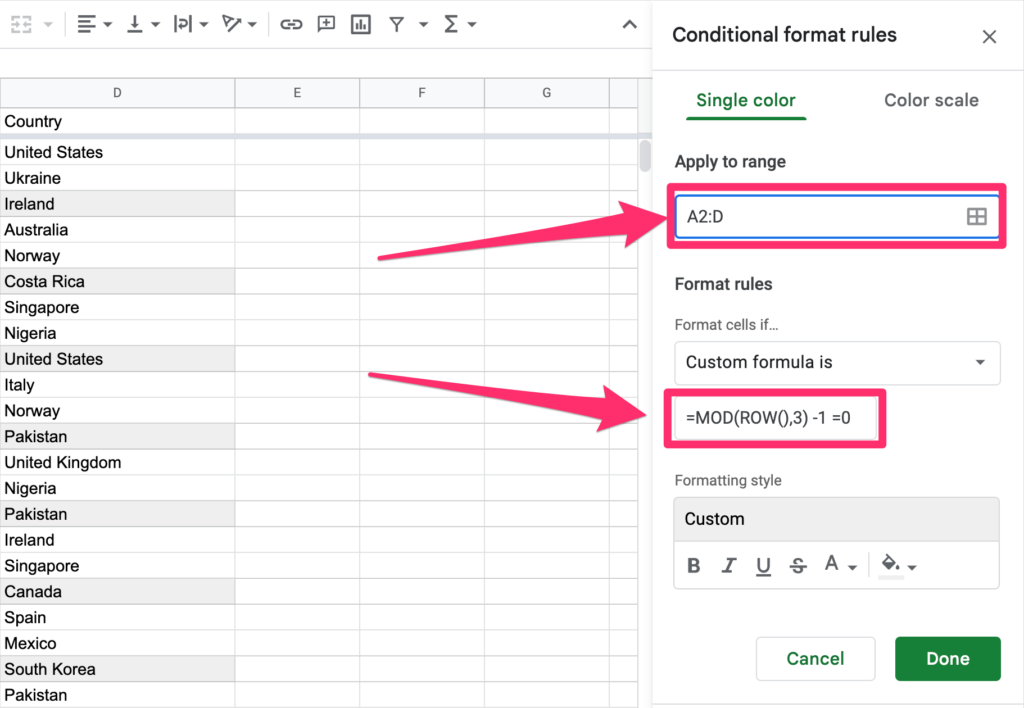
Here’s our updated formula: =MOD(ROW(),3) - 1 =0
Note: This will also apply styles to the header now, so you may also wish to change the range to A2:D
And this is what you should see as the final output you should be seeing:
Example 3: How to add multiple alternating colors in Google Sheets
Adding many alternating colors will be repeating the very same steps we covered in the previous section.
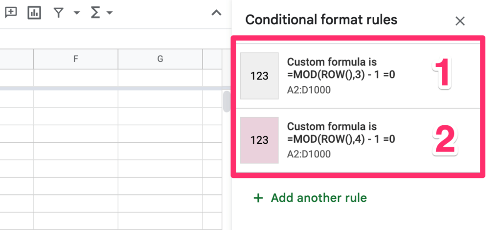
All you need to do is to apply another conditional formatting rule that will just target different cells.
For example, if you want to target every fourth row you need to alter your formula to =MOD(ROW(),4) - 1 =0 and set different formatting options
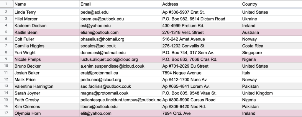
And this is how the final effect should look like:
Example 4: How to add alternating colors based on a value in Google Sheets?
If you want to highlight an entire row where a specific cell contains a specific value, there is a way to do so. We will rely on conditional formatting again and we will also learn a bit about absolute references.
Here’s what you need to do:
Step 1 (Optional): Open the “Exercise 4 – start” worksheet
Step 2: In the Options Menu go to “Format” and select “Conditional formatting”
Step 3: In the pane that you will see on the right-hand side set the range to A1:D to include all rows in the sheet
Step 4: Now, find the “Format rules” section and set the “Format cells if…” to “Custom formula is”
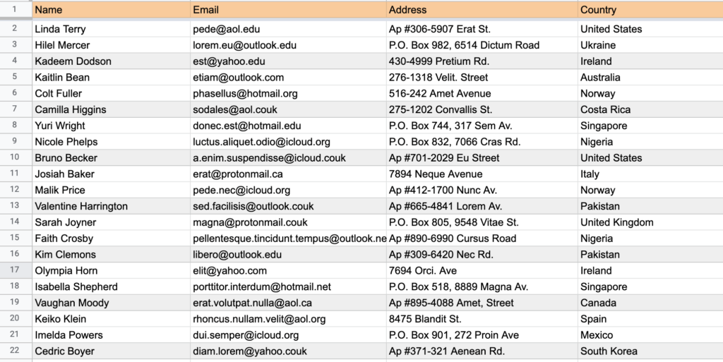
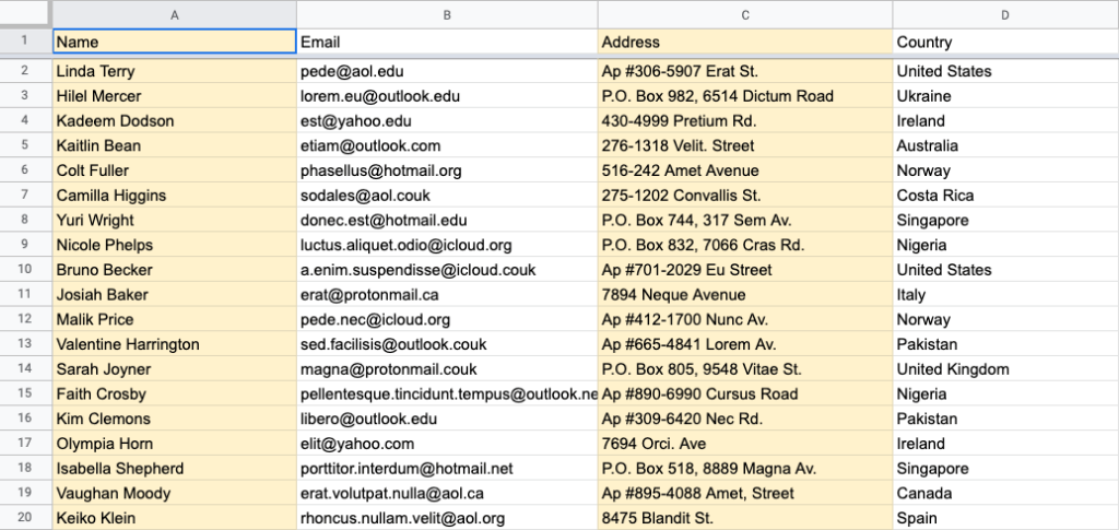
Step 5: Paste this formula into the input that will appear below: = $D2 = "United States" and apply some formatting styles
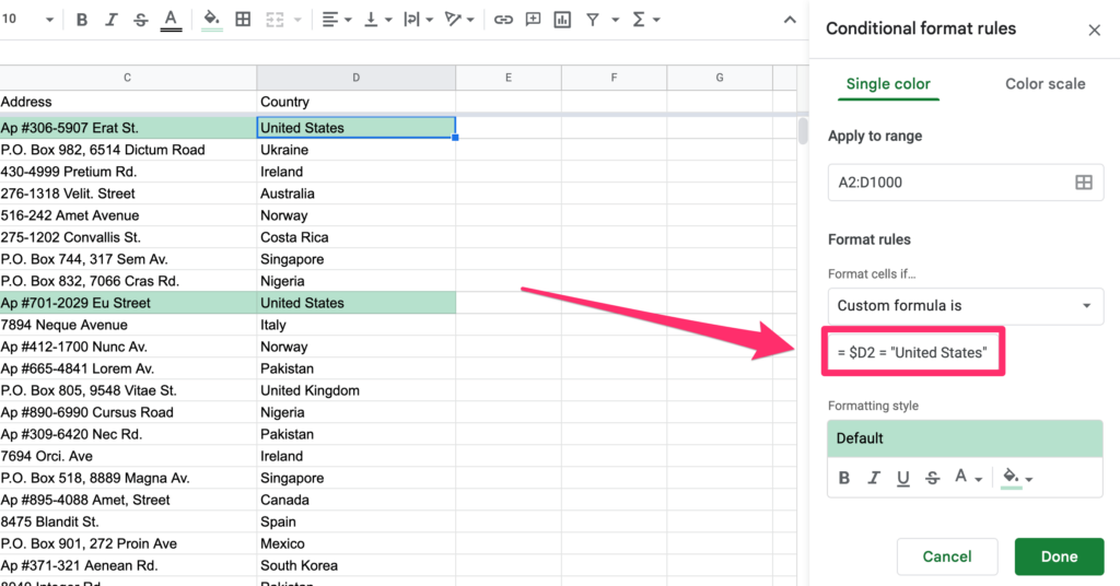
Chances are that you are wondering what the $ sign does. And that’s a brilliant question!
The $ sign before the column name tells Google Sheets to use that specific cell value for all cells in our data set.
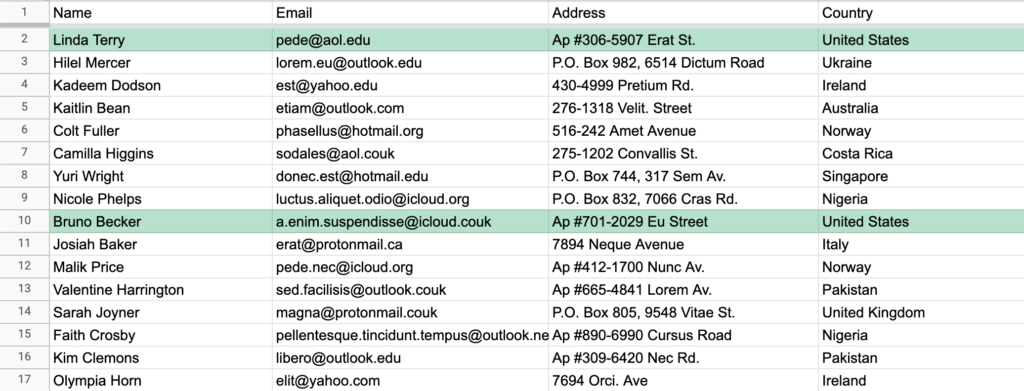
For example, when the parser checks the A2 cell $D2 makes it possible to check the D cell value (which is “United States” and meets our criteria).
Without the $ sign, it would:
- check the cell value (Linda Terry) against “United States” (that we provided in the custom formula field)
- return FALSE.
PS I’ve covered a more complex example of using absolute references in the following article: how to insert and use checkbox in Google Sheets
And here’s the final output of our exercise:
How to Remove Alternating Colors in Google Sheets
As you now know, there are two ways to alternate row colors in Google Sheets:
- using the alternate color option
- or (for more complex use cases) by applying conditional formatting with a custom formula.
The method you choose will affect how you remove colors that are alternate. Yet, the good news is that it will be a quick process either way:
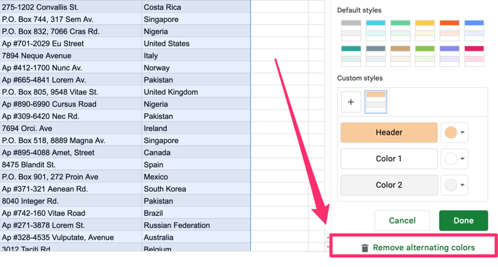
Remove alternating colors created by the “Alternate color” option:
Step 1: In Options Menu select “Format” and then click on “Alternate colors”
Step 2: Remove the existing setting from your worksheet by simply clicking on “Remove alternating colors”
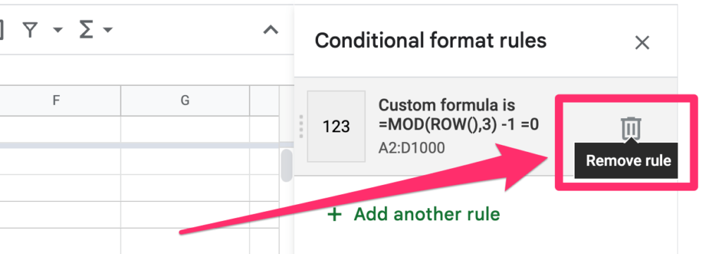
Remove alternating colors created by the “Conditional Formatting” option:
Step 1: Focus on a cell that has the conditional formatting applied
Step 2: From the Options Menu select “Format” and then click on “Conditional formatting”
Step 3: Remove the existing formatting from your worksheet by simply clicking on the trash icon next to your formula
How To Apply Alternating Colors For Columns in Google Sheets
If you want to improve your data’s readability, you’ll usually need to alter row colors.
However, there are some exceptions where you may have to alter column colors instead.
Although that’s not a standard option, there is a way to achieve this effect. Here are the steps you need to follow:
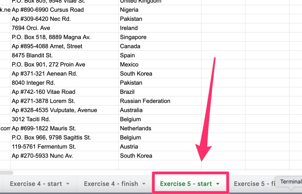
Step 1 (Optional): Open the “Exercise 5 – start” worksheet
Step 2: in the Options Menu navigate to Format > Conditional formatting
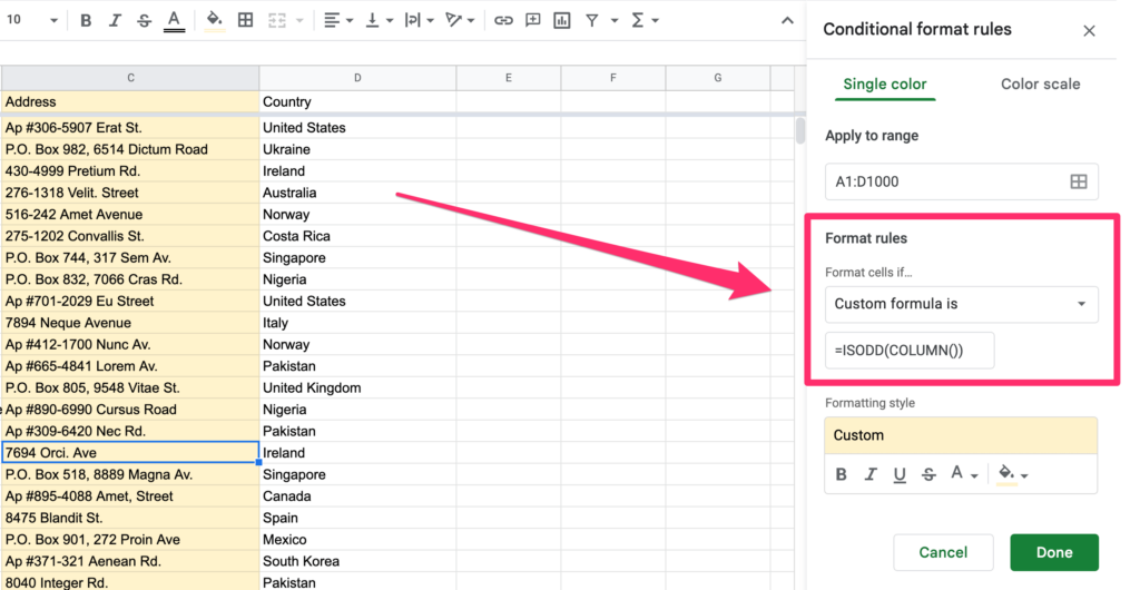
Step 3: In the format rules set the range to A1:D cells and set the “Format cells if…” to “Custom formula is”
Step 4: Add a custom formula to the input field
Use:
=ISODD(COLUMN())if you want to start with the first column (column A)=ISEVEN(COLUMN())if you want to start with the second column (column B)
Step 5: Click on done and check if your formatting is applied correctly
Some Questions You May Still Have
What To Do When Alternating Colors Option In Google Sheets Is Not Working?
If you’ve used the “conditional formatting” and your colors are alternating, it’s likely that the formula is not returning TRUE. If that is happening, double-check the formula to make sure it is returning the correct values
Summary
In this tutorial, we have covered 4 different ways of applying alternate colors to your worksheet.
We went through:
- a way to highlight every other row,
- the idea of how to add banded colors every nth row,
- a way to add multiple alternating colors,
- and how to highlight rows based on a specific cell value.
As you have seen, your options for creating the above are narrowed to two choices. In the simplest scenario the “Alternate colors” will be enough. For some advanced examples, you can use conditional formatting for alternating row colors.
Hopefully, I’ve covered everything you should know, however, if you have any questions feel free to let me know in the comments!