An option to use a custom-defined name instead of referencing cell ranges makes your work smooth like butter, makes the worksheet easier to work with, and easier to understand for others.
This is particularly useful when dealing with complex sheets but not only.
That’s precisely why, in this tutorial, I’ll give you a detailed guide on adding and using named ranges in Google Sheets and show you how you can benefit from it.
I’ll be honest: learning named ranges is a massive game-changer in your daily workflow.
- How To Add Named Data Range In Google Sheets
- How To Use Named Ranges in Google Sheets? (My 4 Ideas)
- How to Edit Named Ranges in Google Sheets?
- How to delete named ranges in Google Sheets?
- How to Create a Dynamic Named Range in Google Sheets?
- How to Create Named Ranges in Google Sheets Mobile App? (Iphone, Ipad, Andorid)
- Some Questions You May Have
- Summary
How To Add Named Data Range In Google Sheets
Adding a named data range in Google Sheets is quite an easy process. Here’s what you need to do:
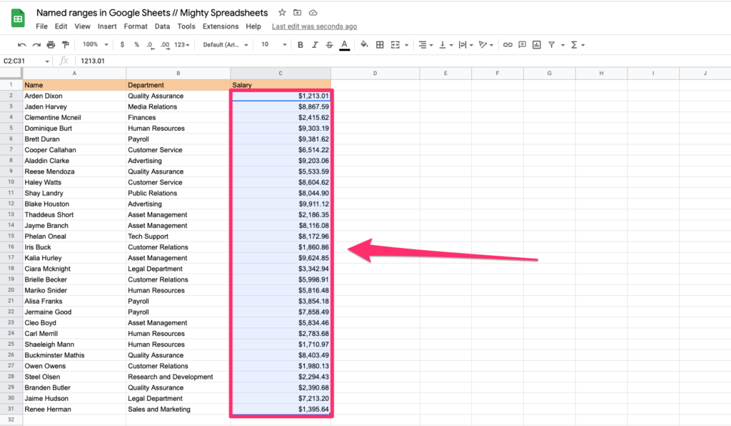
Step 1: Select all cells that you’d like to name
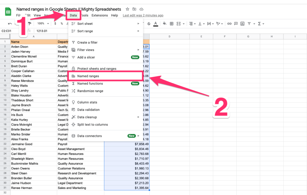
Step 2: In The Options Menu, select Data and then “Named ranges.”
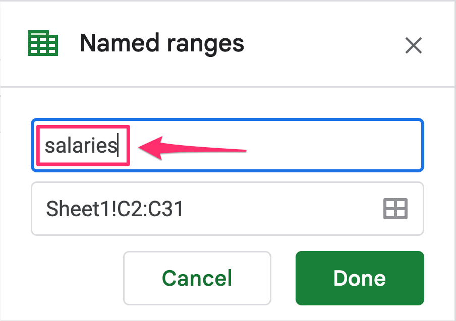
Step 3: In the dialog box type the range name and click on the DONE button
If you want to speed up the process, you can also create a named range with your keyboard. Select the cells you want to name and press Control + J on Windows and Command + J on Mac.
That’s it, and you just created your first named range. 🎉
Before I show you a few examples of how to use a named range in real-life situations, I want to give you some hints about restrictions in creating range names
Rules for creating range names
- Range name is limited to letters, numbers, and underscores only.
- It must not exceed 250 characters.
- You can’t start with a number.
- You can’t start with words ‘TRUE’ or ‘FALSE.’
- Named range can’t mimic regular range naming (i.e., A2:D4 is not a valid name for a range)
How To Use Named Ranges in Google Sheets? (My 4 Ideas)
1: Use Named Ranges in Functions
Using named ranges is almost as easy as creating them. Just pick a function that takes a cell or a range of cells as an argument and type your range name inside.
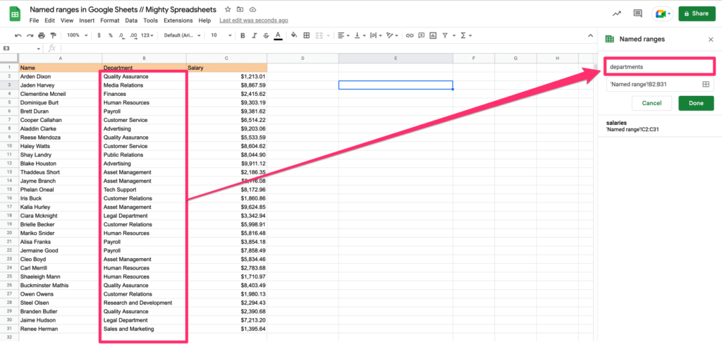
Let’s have a look at this sheet below.
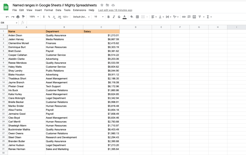
You can see a list of names, departments, and salaries. Let’s focus on the last column.
If you want to perform calculations without using a named range feature, you would need to use a C2:C31 range as a reference.
But to save us a bit of time, let’s name it (surprisingly) “salaries”.
Now whenever you want to refer to those cells, you can use their names
For example:
=SUM(salaries)=AVERAGE(salaries)
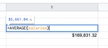
and so on.
2: Create Drop Downs with Named Range Data Validation
If you want to display Named Range data as a drop-down, there’s an easy way to do it. Here’s what you need to do:
Step 0: Following the steps from the first section create a new range named “department” (from B2:B31 cells)
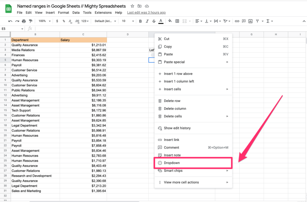
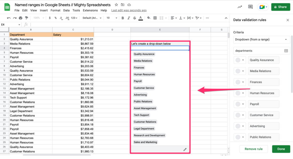
Step 1: Right-click on the cell where you want the drop-down to appear and select “Dropdown” from the context menu
Step 2: You will see a dialog box on the right-hand side. In the “Criteria” section, please select the “Dropdown (from range)” option.
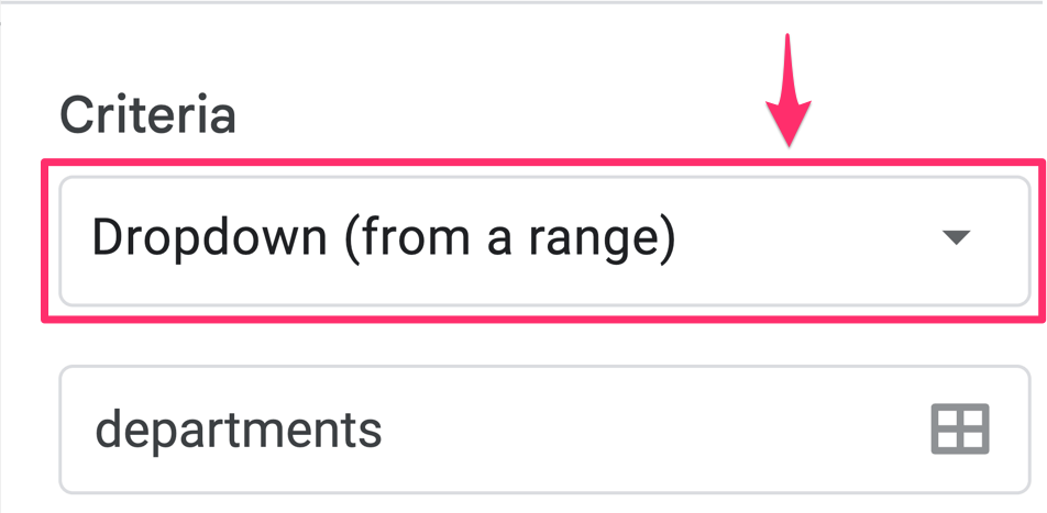
Step 3: Instead of providing a range, manually enter your previously defined range name
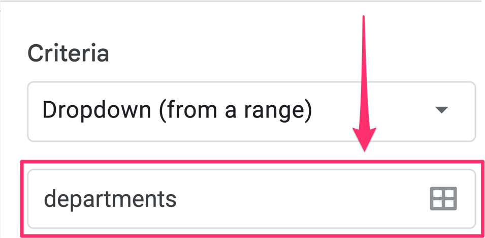
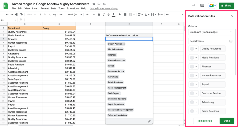
Step 4: Click on the DONE button, and all the items will be available in the dropdown
You can learn more about drop-downs in this article: how to make drop-down options in google sheets
3: Use Named Ranges in Hyperlinks
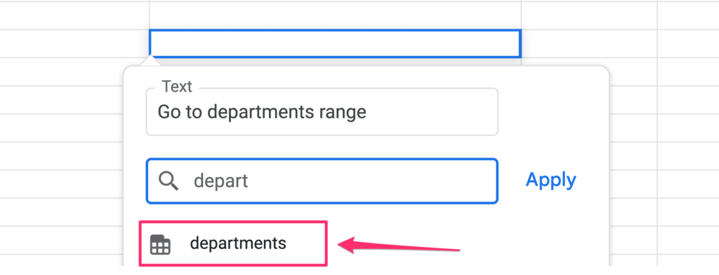
When creating hyperlinks to another tab, you can refer to the named range rather than the regular range of cells.
Make sure to check this article if you want to learn more about different ways to link to Google Sheets
4: Use Named Ranges with App Scripts
Creating named ranges also makes it much easier to use when using App Scripts. You can easily pull data from named ranges using multiple functions described in docs. Here are a few that I like the most:
getNamedRanges()[gets all the named ranges defined in the document]setNamedRange()[allows to create a range dynamically]getRangeByName()[gets provided range so you can perform any operation on it]removeNamedRange()[to delete any range you want]
How to Edit Named Ranges in Google Sheets?
That’s a prevailing situation. Your spreadsheet has changed and has more or fewer entries, and you need to adjust the named range to reflect the new data state.
Or the data context has changed, and you need to rename your range.
How can you do that?
Don’t worry. It’s pretty easy as well. Here are the steps you need to cover:
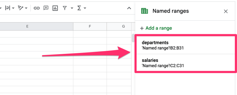
Step 1: In the Options menu, select Data > Named ranges
Step 2: On the right side of your screen, you’ll spot a dialog box with all sheet ranges clearly outlined.
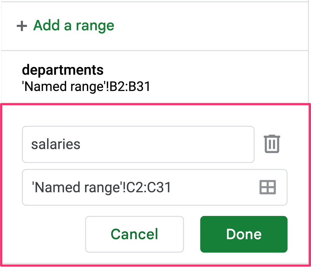
Step 3: Hover over the range you need to edit and click on the pencil icon.
Step 4: This will allow you to change the range name or update the scope of the range.
How to delete named ranges in Google Sheets?
The process of deleting a named range is quite similar to editing it:
Step 1: In the Options menu, click on Data > Named ranges
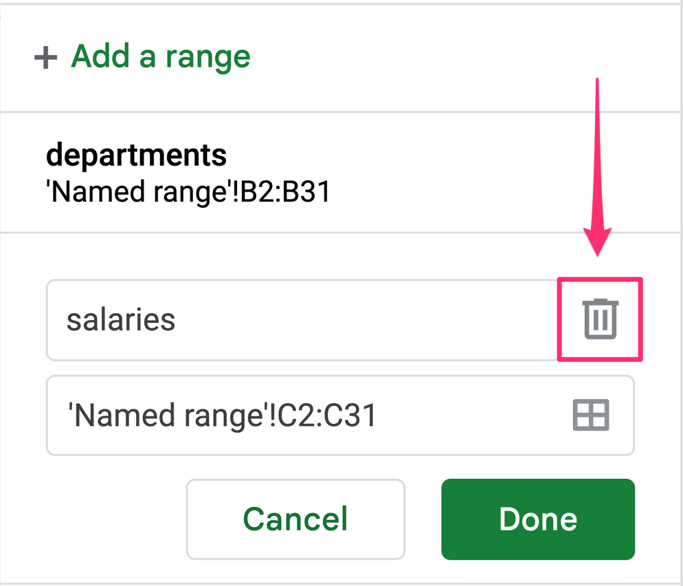
Step 2: Look at the dialog box on the right-hand side of the screen and pick the range you’d like to delete (hover over and click on the pencil icon)
Step 3: Look for the trash icon next to the range name input field. Click on it, and the range will be gone.
How to Create a Dynamic Named Range in Google Sheets?
When you create a named range, you will see no option to provide a formula-based range name. A range that would be dynamic and would take a dynamic parameter.
Hence you may be thinking that named ranges in Google Sheets are static. And you are possibly correct; however, there’s a trick to making a range dynamic using the INDIRECT function.
Here’s how you can do it:
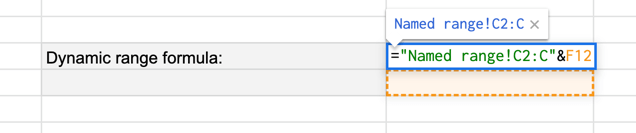
Step 1: Create a simple formula that contains a range reference built from a string and a dynamic value taken from another cell:
="Named range!C2:C"&F12
Where:
- “Named range” is the name of our worksheet tab
- C2:C – is a static range
- F12 – is a reference to the F12 cell value. The value of the cell will define the range that is used.
Step 2: Create a named range for this cell. Let’s name it “dynamicNamedRange”
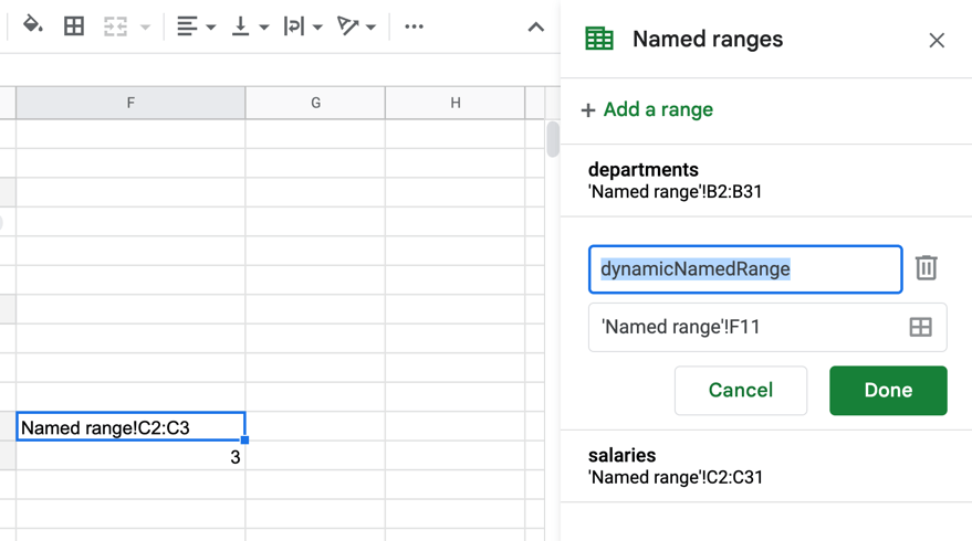
Step 3: Refer to the dynamic range by using the INDIRECT function
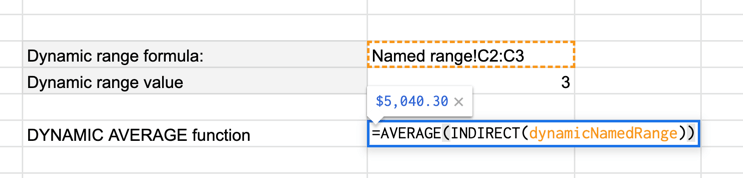
Example: =AVERAGE(INDIRECT(dynamicNamedRange))
Dynamic range in action:
How to Create Named Ranges in Google Sheets Mobile App? (Iphone, Ipad, Andorid)
At the moment of writing the article, this feature cannot be used on iPhone or iPad devices.
When using Android devices, the capability for working with named ranges is present but limited. You can only select previously (on a computer) created named ranges, but you can’t edit them or create new ones.
Some Questions You May Have
Can you name a cell in Google Sheets?
Yes, you can name a cell in Google Sheets. To achieve this, pick one cell, select Data > Named ranges from the options menu, and name the cell as you wish.
Can you reference a column in a named range?
Yes, you can reference a Column inside a named range using the INDEX function, which will find and list values from a selected range. For example, your code could look like this: =INDEX(your_range,0, 2) – if you refer to the second column.
How to solve the “unknown range name” error in Google Sheets?
The unknown range name error is usually caused by a typo, extra space, or extra character that accidentally got into your formula. I recommend checking it once again or even trying to rewrite it from scratch.
If it doesn’t help, that means that the formula itself is correct, but the source of the issue may lie in one of the cells. That would mean you must check all the cells for invalid values.
How to create a named range in multiple discontiguous columns?
Although it sounds like a great idea, there is no support for non-adjacent cells/columns in Google Sheets.
Summary
I hope that now you at least feel familiar with using named ranges in google sheets. They are an essential tool for organizing and manipulating data in Google Sheets. They provide the ability to give meaningful names to a specified range of cells, making it easier to work with formulas and app scripts.
Users can reference a range of cells with named ranges without remembering cell coordinates. This makes working with spreadsheets more efficient and reduces the risk of errors.
What is your favorite way to use named ranges? Let me know in the comments!