How To Clear Cell Contents In Google Sheets? (4 Different Ways)

Posted on July 28, 2023August 1, 2023 by Luke

We all know that we can simply delete the values in any spreadsheet just by pressing the “Del” button on our keyboard. But, at times, you may need some more controls. And there are many ways available to clear cell contents in Google Sheets.

To delete just values, select your cell range first and then “Edit>Delete>Values” to clear it. And to delete the formatting too, select the range again and then “Format>Clear Formatting” to clear it. You can also use the backspace button or the “Ctrl + \” shortcut to do the same. And for a more complex deletion process, you can use “Apps Script” as well.

Depending on the type of deletion you are looking for, such as deleting the values while keeping the formatting or deleting the formatting while keeping the values, you need to use different methods in Google Sheets. So, I’m going from the easiest to the most complex one!

How To Clear Cells In Google Sheets? (4 Methods That I Use)

Depending on your requirement, you can delete any data or cell content in Google Sheets in various ways, such as by keeping the formatting intact.

There are four distinct methods available in Google Sheets that can be a lifesaver in need.

Method 1: Delete Cell Contents Without Shifting, With The “Delete Values” Option

You must have seen that when you try to delete an entire row in Google Sheets to clear cell contents, it automatically deletes the complete row and shifts the lower row to that place.

With a little tweak, you can do it without even shifting the cells. The steps are pretty simple, though!

Step 1: Launch Google Sheets and open the spreadsheet.
Step 2. Select the entire cell range that you want to delete (Either by dragging the mouse or by Shift + click).

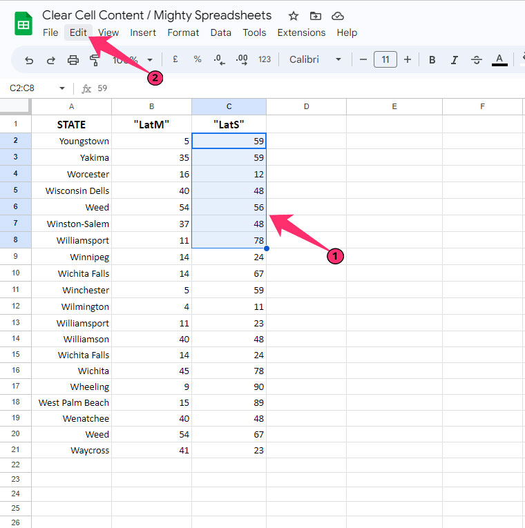
select cell range and click on edit button

Step 3: Navigate to the menu bar and click on the “Edit” button.
Step 4: Hover your cursor over the “Delete” option, and a floating menu will appear.

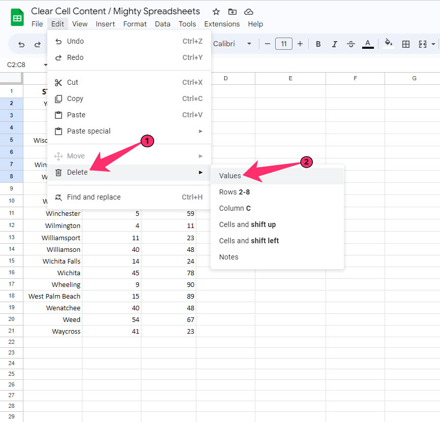
Delete values under edit button in sheets

Step 5: Click on the “Values” option.

You can now see that the entire value is deleted from the selected cell range without shifting the bottom row.

But there is a catch! This operation will keep the formatting for that particular cell range even after deleting the values.

There is a workaround by which you can also delete the formatting too!

Step 6: Select the same cell range.

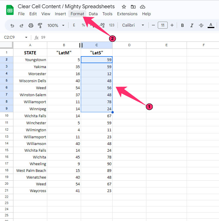
select cell range and click on Format button

Step 7: Navigate to the menu bar and click on the “Format” button.
Step 8: Once the drop-down menu appears, click on the “Clear Formatting” option.

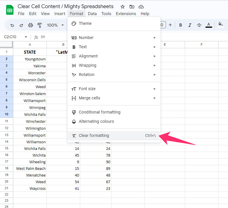
Step 9: Alternatively, you can use the “Ctrl + \” shortcut.

Even if you clear both the values and formatting in this way, it will not shift any row or columns. If you are working with complex data, it can be a lifesaver!

Note: Not just values or formatting, you can now also find and remove duplicate values and texts in GS with a few simple steps.

Follow my latest 2023 blog on removing duplicates in Google Sheets to know more!

Method 2: Clear Content With A Keyboard Shortcut

If you want to delete any simple data from any cell, or even cell range, you can also do it by using shortcuts. To clear just the content, select the cells first and then hit the backspace button. It will only remove the value but not the formatting.

If you are looking for some advanced deletion option, there are two shortcuts available on Google Sheets that are truly useful.

Operation	Windows Shortcut	Mac Shortcut	Google Chrome Shortcut	Other Browser Shortcut
Delete Row	Ctrl + Alt + –	⌘ + Option + –	Select the rows to delete.Press “Alt + E”Press “D”	Select rows.Press “Alt + Shift + E”Press “D”
Delete Column	Ctrl + Alt + –	⌘ + Option + –	Select the columns to delete.Press “Alt + E”Press “E”	Select columns.Press “Alt + Shift + E”Press “E”

If you are working in Google Sheets on the Safari browser on your Mac device, you can open the advance deletion menu by pressing “Ctrl + Option + E” altogether. Then press “D” to delete rows and press “E” to delete columns.

Note: If you are working with a complex spreadsheet with loads of data, you need to zoom in and out to search and register any particular data.

Don’t forget to check out my newest guide on how to zoom in and out in Google Sheets.

Method 3: Clear Cell Contents By Removing An Entire Row Or Column

If you want to delete any cell range (in rows or columns) where the next row or column will automatically shift, you can easily do it by deleting the entire row or column.

Step 1: Launch Google Sheets and open the spreadsheet.
Step 2: Click on the header name (row or column) that you want to delete.
Step 3: Right-click on the header name to fetch the contextual menu.

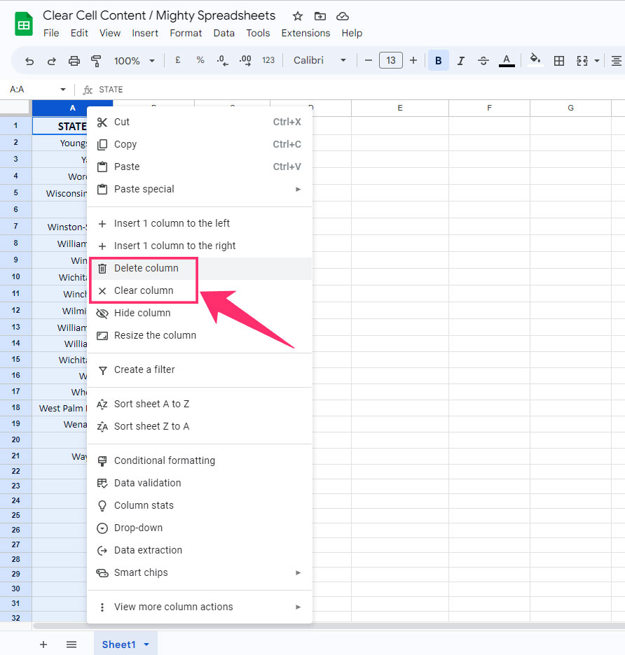
Delete Column and clear column button in sheets

Step 4: Click on “Delete Column” or “Delete Row” to remove it entirely.
Step 5: If you want to keep the row or column but want to delete just the values, click on the “Clear Column” or “Clear Row” option.

If you don’t want to delete the entire cell or the values but need to remove it to work with other cell ranges without it, you can do it by clicking on the “Hide Row” or “Hide Column” options.

Bonus: Google Sheets now gives you the option to collaborate with other people in real time. And this option is truly useful if you are working as a team on a complex spreadsheet.

To know more, follow my latest blog about how to share and collaborate in Google Sheets.

Method 4: Clear Contents Using Apps Script

If you need an advanced deletion method where you can keep the formatting while deleting the values or keep the values while deleting the formatting, you can easily do it with Apps Script.

Step 1: Launch Google Sheets and open your spreadsheet.
Step 2: Navigate to the header menu and click on the “Extensions” button.

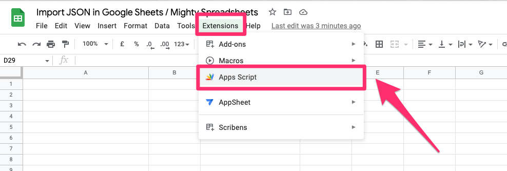
Step 3: Click on the “Apps Scripts” option, and a new page will open.
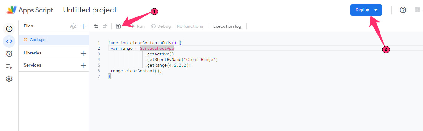
Step 4: Now, enter the code as it is.

function clearContentsOnly() {
 var range = SpreadsheetApp
               .getActive()
               .getSheetByName("Clear Range")
               .getRange(4,2,2,2);
 range.clearContent();
}

Step 5: Click on “Save project” and then on the blue “Deploy” project.

Step 6: Give necessary permissions and run the Apps Script code.

Note: I’ve included the cell range in the “getRange” section in the code. You need to replace that parameter and include the cell range which you want to delete. But it will delete just the values while keeping the formatting as it is.

It is also possible to clear the formatting while keeping the value intact by using Apps Scripts.

Step 1: Launch Google Sheets and navigate to the Apps Script page.
Step 2: Enter the following code.

function clearFormattingOnly() {
 var range = SpreadsheetApp
               .getActive()
               .getSheetByName("Clear Range")
               .getRange(4,2,2,2);
 range.clearFormat();
}

Step 3: Click “Save project” and then “Deploy” it.
Step 4: Give permissions and run the project to keep the values while removing the formatting.

Note: Like the previous script, I’ve included the cell range in the “getRange” section. Change the values according to your cell range.

Bonus: Do you know that you can now easily integrate date functions in Google Sheets? Check out my newest guide on using the date functions in Google Sheets to know in detail.

How To Clear Contents In Google Sheets Without Deleting Formulas?

If you delete any cell content, it will automatically delete the formulas attached to them (not formatting). And there is no way to keep the formulas intact while deleting the values or texts from the respective cells. But there is a workaround!

You can simply use the “Named function” option to generalize your formula. Once you do that, you can easily recall the formula. The steps are very easy!

Step 1: Launch Google Sheets and open the spreadsheet.
Step 2: Right-click on the cell that has the formula to fetch the contextual menu.

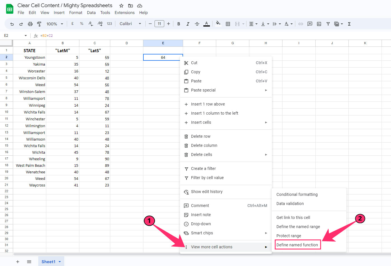
Step 3: Hover your mouse over the “View more cell actions” option.
Step 4: From the side-loaded menu, click on the “Define named function” option.
Step 5: On the right-side menu, definite the name of your formula in the “Function name” field.

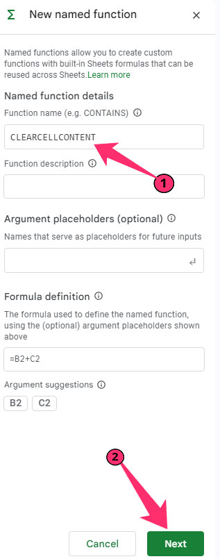
Step 6: Enter “Function description” and “Formula definition” in the respective fields.
Step 7: If your formula has an argument, define that in the “Argument placeholder” field.
Step 8: Click on the “Next” button to check the preview of your named function.
Step 9: Tap on the “Create” button to save the function.

Once you create a named function, you don’t need to write the entire formula every time. You can simply recall the formula by putting its name in the function (fx) field.

Note: Not just functions, you can now even name an entire cell range to generalize it. It will also make it easier to use the entire cell range in any formula using just the name assigned. To know in detail, check out my guide on named ranges in Google Sheets.

Final Note

Until you need more customization and control over your deletion process, especially while working with complex data, just use the “Delete” or “Backspace” button on your keyboard, which will serve your purpose. But for advanced controls, you have to use other ways.

If you are working with a considerably vast cell range, it is better to use the Apps Script, as you can define the entire cell range and get it done in a second. So, that’s all for today, geeks! Feel free to drop your queries and start a conversation with me in the comment section below!