We generally use Google Sheets to access our complex spreadsheets that often involve a huge amount of data with complex formatting. And it is tough to search for any particular string manually on Google Sheets. But yes, there are workarounds!
Using the “Find” option by pressing the “Ctrl/Cmd + F” is the easiest one to search for anything on Google Sheets. You can also use the “Find and replace” and the “Conditional formatting” option. And for more complex spreadsheets, the “FIND,” “SEARCH,” and “MATCH” functions can also be used.
Although “Find” is the easiest way to search for anything on GS, it is not very versatile. On the other hand, complex functions like “MATCH” can be a little tough to work with for newbies, but it is one of the most versatile ones. So now, we will look at all the possible methods.
How Do You Search In Google Sheets: Six Methods I Use At Work
Not one or two, but there are six different methods available to find or search any string on Google Sheets. So, I’m going from the easiest to the most complex one.
Method 1: Use The “Find” Option
Similar to other Google Workspace apps, Google Sheets also come with an inbuilt “Find” option. Although it is not quite versatile, especially in complex spreadsheets, it can be a handy tool for you if you just want to highlight any particular string you are searching for.
The steps to search on google sheets using the “Find” option are as follows:
- Step 1: Launch Google Sheets and open your spreadsheet.
- Step 2: Press “Ctrl + F” on Windows and “Cmd + F” on Mac.
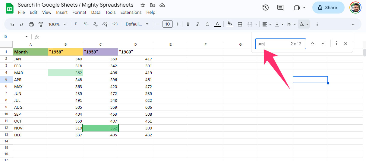
- Step 3: Navigate to the small popup box in the top-right corner.
- Step 4: Enter the string (text or value) in the “Find in sheet” field.
- Step 5: It will automatically highlight the matching cells in green color while giving you a count of matching strings.
- Step 6: Use the “Up” and “Down” arrows on the popup box to navigate to the next matching cell.
This simple “Find” option will highlight those cells if it contains the search string, even in a sentence. Suppose you are searching for “Apple,” then it will also highlight cells containing “Pineapple,” as it can find “Apple” in this word. And due to that, this function is not recommended for complex spreadsheets.
Note: With this “Find” feature, you can now also find duplicates in your spreadsheet. To know more with a hands-on guide, check out my latest tutorial on removing duplicates in Google Sheets efficiently.
Method 2: Use The “Find And Replace” Option
The “Find and Replace” tool is way more versatile than the “Find” feature on Google Sheets. You can either directly replace it with a new value or can just search for a particular string with this option.
Here are the steps to search on Google Sheets using the “Find and replace” option.
- Step 1: Click on the “Edit” button on the header menu of your spreadsheet.
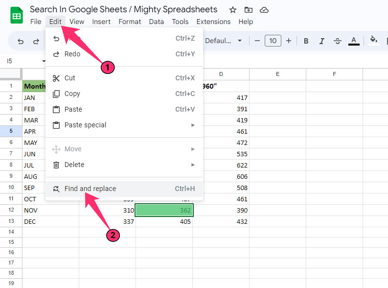
- Step 2: Click the “Find and replace” option (Alternatively, use the “Ctrl + H” or “Cmd + H” shortcuts).
- Step 3: This will automatically bring a popup box.
- Step 4: Enter the string you are searching for in the “Find” field.
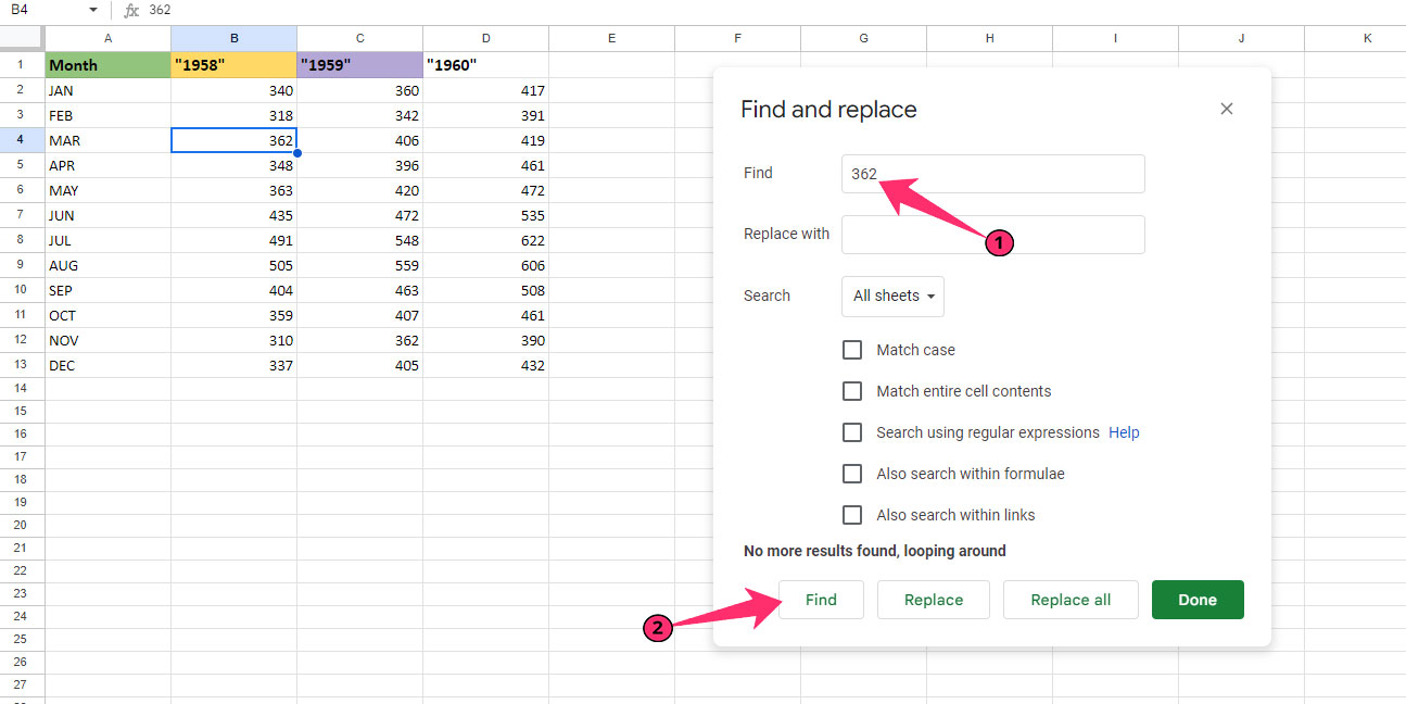
- Step 5: Click on “Find,” and it will automatically highlight the first matching cell.
- Step 6: Click on “Find” again to search for the next matching cell.
- Step 7: Once you reach the last matching cell for your searching string, you’ll get a “No more results found, looping around” message on the popup box.
- Step 8: Click on the “Done” button to close the “Find and replace” box.
If your spreadsheet contains multiple sheets, but you want to restrict the search for the sheet you are working on, simply click on the dropdown menu beside the “Search” option and select the “This sheet” option. You can also define a particular range by selecting the “Specific range” option.
Note: If you want to replace your searching string with a new string in your spreadsheet, enter the searching string in the “Find” field and the replacement string in the “Replace with” field. Click on the “Replace” button to replace individually or “Replace all” to replace all the matching strings at once.
Bonus: At times, you may need to check the edit history of your spreadsheet, especially if the spreadsheet is shared by a team where multiple people work on the same spreadsheet. But don’t worry, have a look at my newest blog on how to see edit history in Google Sheets to know more!
Different Filters Of The “Find And Replace” Option
As of April 2023, Google Sheets gives you five different filtering options in the “Find and replace” tool. And depending on your specific needs, you can use these particular filters to get a refined result.
The current filters and how they actually work.
#1. Match Case
This filter makes your search case-sensitive. So, if you are searching “Ronaldo” while using this filter, it will automatically ignore those cells even if they contain “ronaldo” in lowercase. This filter is particularly helpful for text searches.
#2. Match Entire Cell Contents
With this one, you can search for the exact term. Suppose you are searching for “Ronaldo” with this filter; it will ignore the cells containing the “Cristiano Ronaldo” term. Although “Cristiano Ronaldo” contains the search term “Ronaldo,” it is not the exact one in the entire cell; thus, this filter ignores it.
#3. Search Using Regular Expressions
This filter will help you search with regular expressions of formula. By using this filter, you can search for the exact output while using the formula as a search term.
Suppose you want to search all the uppercase words in your spreadsheet; you can do that by entering the “^[A-Z].*” search term while using this filter. It will automatically find all the text strings that start with an uppercase.
Note: Google uses RE2 for all the regular expressions. You can find more details on Google’s regular expressions on the RE2 GitHub page.
#4. Also Search Within Formulae
The normal “Find” function will search the output of a formula in a cell rather than the formula itself. But if you want to find anything in a particular formula, you can now even do that by using this filter.
#5. Also Search Within Links
By using this filter, you can now even search links attached to a text string in your spreadsheet. So if you have a name in the A1 cell and an attached link for that text in the B1 cell, you can find the links just by searching the name while using this formula.
Note: You can now share your spreadsheet and collaborate with your team members in real-time on Google Sheets. Check out my detailed guide on how to share and collaborate to know more!
Method 3: Use Conditional Formatting
All the search functions we have mentioned above can only highlight matching cells one at a time. But it can be painstakingly difficult to operate if you are working with a large spreadsheet.
By using the conditional formatting option, you can now also highlight all the matching cells at once.
- Step 1: Click on “Format” from the header menu.
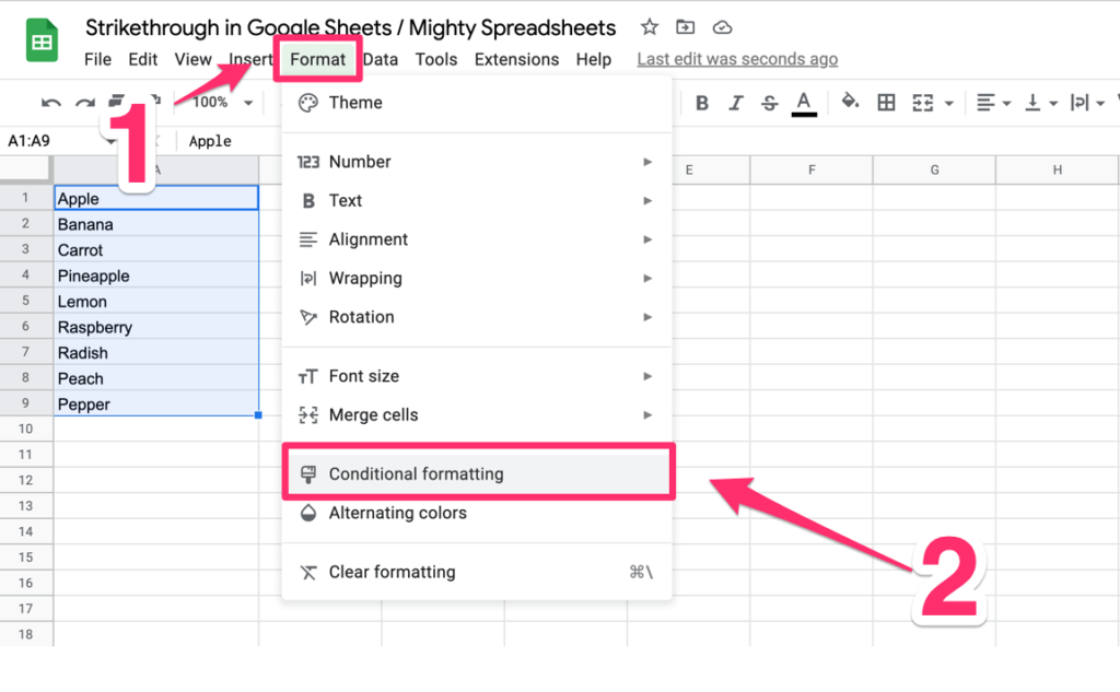
- Step 2: Click on the “Conditional formatting” option.
- Step 3: You can now find a sidebar named “Conditional formal rules” on the right-hand side of your spreadsheet.
- Step 4: Select “Single color” from the header selection tab.
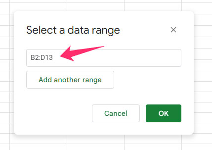
- Step 5: Define the search range in the “Apply to range” box and click “OK.” (Alternatively, click and drag your selection, and it will automatically define the selected range)
- Step 6: Click on the dropdown menu beneath the “Format cells if…” option.
- Step 7: Select “Text contains” if you want to search for a text string.
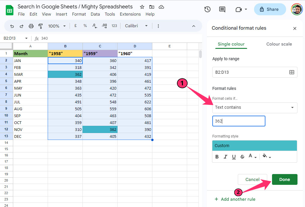
- Step 8: Enter your search term in the “Value or formula” field.
- Step 9: Click on the fill color icon on the “Formatting style” field.
- Step 10: Define the color that you want for highlighting all the matching cells.
- Step 11: Click on the “Done” button, and all the matching cells will be highlighted in your defined color at once.
Example: Suppose we want to highlight all the cells in green that contain the “Ronaldo” text string. By using your entire sheet in the “Apply to range” field and defining the green color in the formatting style, you can highlight all the cells containing the “Ronaldo” word at once.
Bonus: You can now filter data in Google Sheets very easily, even if you are working with a very complex spreadsheet. Check out my 2023 guide to filter data to know the details!
Method 4: Use The “FIND” Function
There are two specific functions already available in Google Sheets by which we can search any string. You can even search a particular string on another specific string by using the “FIND” function. (E.G., you can search the content of “B1” in “A1” while defining just the cells rather than actual search terms.)
The main formula is “=FIND (<Search term>,<search range>)” (you can also add another modifier at the end to define a cell from where you want your search to start).
Here, we have a sentence, “Argentine star Lionel Messi plays for French side PSG” in the A1 cell. And we have “Messi” (our search term) in the B1 cell. Now, we want to search for the B1 string in the A1 cell. So, the steps are:
- Step 1: Open the spreadsheet and click on an empty cell where you want your output.
- Step 2: Click on the Function (fx) field.
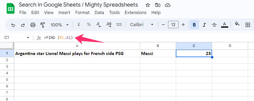
- Step 3: Put the “=FIND (B1,A1)” formula and hit the enter button.
- Step 4: You’ll get “23” as the output in your selected cell.
Explanation: This function will not highlight the matching strings. Instead, it will give you a count for the position from where your search string starts at the matching string. Here, our search term “Messi” starts from the 23rd position (including spaces) in the actual sentence. Hence, we get “23” as the output.
Remember that it is a great technique to search for a word in Google Sheets, although it is case-sensitive. So, include the case-sensitive search term to get the right output. You can now also capitalize the first letter in Google Sheets with a few easy steps.
Method 5: Use The “SEARCH” Function
The “SEARCH” function works similarly to the “FIND” function that helps you to search on Google Sheets. Besides, both these functions have the same parameters.
The formula is “=SEARCH (<Search term>,<search range>)” (Like the “FIND” function, you can also add a modifier at the end to define from which cell you want the search to start).
We will now again try to search “Messi” in the “Argentine star Lionel Messi plays for French side PSG” sentence. The steps will be,
- Step 1: Select the cell where you want your output (here, it is C1).
- Step 2: Click on the function (fx) field.
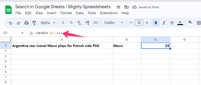
- Step 3: Use the “=SEARCH (B1,A1)” formula and press enter.
- Step 4: You will see 23 in the C1 cell as the output.
Again, we will see the starting position rather than a highlighted cell as the output of this function. It is also a case-sensitive function like the FIND one.
Note: It is better to lock the cell range in Google Sheets if you are working on a complex spreadsheet. Don’t forget to have a look at my newest guide on how to lock ranges in Google Sheets to know in detail.
Method 6: Use The “MATCH” Function
The “MATCH” function is the most versatile one that you can use to search for anything on Google Sheets, even on a complex spreadsheet. You can define a range and also a particular order in this function.
The main formula is “=MATCH (<search term>,<search range>,<data order (1 or 0)>” (This is a unidirectional search range that means you can either select or a column. Selecting a two-dimensional array in the search range will return errors).
- Step 1: Launch Google Sheets and select an empty output field.
- Step 2: Click on the function (fx) field.
- Step 3: Enter the “=MATCH (<search term>,<range>,<1 or 0>” formula (Use 1 when the data is in ascending order or use 0 when the data is not in any particular order).
- Step 4: Hit the enter button, and it will give you the position of the matching term in the cell range as the output.
If it shows “2” as the output, it means that the search term you have defined is in the second place from the beginning of your selected search range.
Bonus: It is necessary to use named ranges in a complex formula rather than defining each cell. And to do that easily, follow my latest tutorial on named ranged in Google Sheets.
How To Search In Google Sheets Mobile App (iPhone, iPad, Android)?
If you are using the Google Sheets app on your handheld devices, such as Apple or Android devices, it is better to use the “Find and replace” to search for anything. The steps are pretty easy.
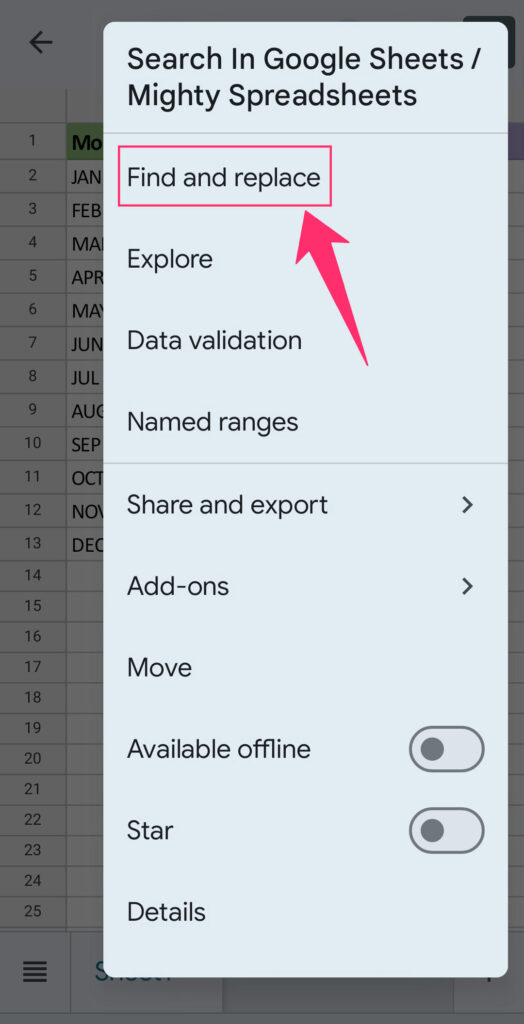
- Step 1: Launch the Google Sheets app and open the spreadsheet.
- Step 2: Tap on the “More” button (three horizontal dots on Apple devices and three vertical dots on Android devices).
- Step 3: Tap on the “Find and replace” option.
- Step 4: Enter the search term in the designated field.
- Step 5: Tap on the “Search” button, and it will highlight the first matching term.
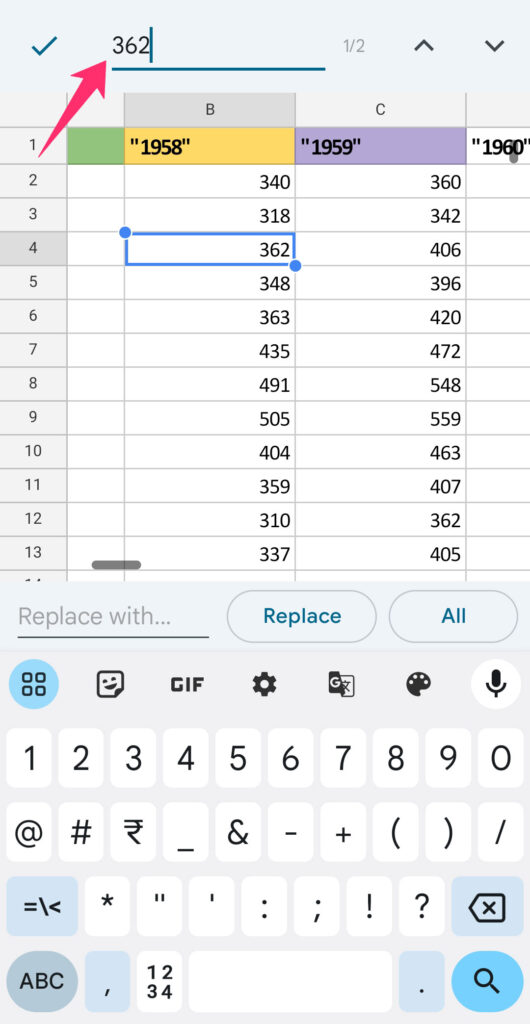
- Step 6: Tap the arrows on the top-right corner to select the next matching string and so on.
- Step 7: Once done, hit the “Close” (X) button to return to the spreadsheet.
Note: If you are working on a large data set on your Google Sheets app, zooming in and out will give you more freedom to focus on a particular range. And to do that easily, follow my latest guide on zoom in and out on Google Sheets.
Final Note
If you are searching for any particular word, such as the surname of a customer, in your invoice, it is better to use the simple “Find” tool to highlight the matching strings one at a time. But for a more complex invoice with multiple clients with the same surname, it is better to use conditional formatting.
In that way, you can easily highlight all the matching cells at once to make it easier for you to work with. But if you are working on a large spreadsheet with raw data and alphanumeric strings, it is better to use the “SEARCH” or “MATCH” function.