Modulo or modulo operator or simply the MOD operator is a highly versatile function in Google Sheets. It is useful as a standalone operation for any simple calculation. Besides, you can also use it inside a complex formula as it perfectly synchronizes with other functions.
The MOD function is basically used to find the remainder of a calculation when you divide a number by another one. While the “Divide” function helps us find the integers, the MOD function solely concentrates on the remaining values after a division.
So now, we will see how we can use this function as a sole operator and will also learn how to use it in a complex formula with other functions. Without any further ado, let’s start!
Understanding Modulo In Google Sheets
Modulo, or the MOD function, is one of the vital functions in Google Sheets. It is not just a unique function to find remainders in any mathematical calculations, but it is equally versatile when used with other functions.
How Modulo Functions Work In Google Sheets?
The Mod function is mainly used to find the remainders in Google Sheets. But to start with, you need to know about the general syntax first.
The formula is “=MOD(<Dividend>, <Divisor>)” to activate the modulo operator.
Here, the “Dividend” is the main number that you want to divide by the divisor. And the “Divisor” is the number with which you want to divide the dividend.
Let’s understand this function with an example. Suppose you want to divide “15” by “4” and find the remainder. So, you need to use the “=MOD(15, 4)” formula, and it will return 3.
Here, the modulo operator first divided 15 (dividend) with 4 (divisor). And then, it calculates the remainder, which is 3, and gives it as the output.
Besides the integer numbers, you can also put non-integer numbers, such as decimals, in this function. Moreover, it can also be used with logical functions like “IF,” “OR,” and “AND.”
Bonus: It is true that the “IF” formula works like a charm with the “MOD” function in GS. To know more, check out my latest guide on using the “IF” function in Google Sheets the right way!
Usage Of The Google Sheets Mod Operator
The modulo operator, or the mod operator, or the MOD, is a versatile function that I’ve already told you about. And before we see the real usage, you need to first know how to access it. There are two ways.
Firstly, you can click on the output cell and then start with the “=MOD” in the function field to activate it. And secondly, you can click on the “Insert” option followed by the “Function” option.
Then, click on the “Math” function and finally select the “Mod” function from the list.
I’ve already shown how to find the simple remainders using this function. But you’ll only see the real usage of this MOD function when you use it in any complex calculation. So, let’s try it.
Example: Let’s say I want to find the remaining days for the month after 17th June 2023. So, you need to use the “MOD” function along with the “EOMONTH” and “DAY” function to calculate this.
The formula will be “=MOD(EOMONTH(“2023-06-17”, 0) – “2023-06-17”, DAY(EOMONTH(“2023-06-17”, 0)))” here. And it will return “13” in the output cell.
Modulo Function In Google Sheets (With Examples)
Modulo or the MOD function can be used as a standalone function, or you can also use it with other functions to perform complex operations. Let’s try to analyze this operation a bit more with some examples.
Google Sheets Mod Function
The syntax of the modulo function in Google Sheets is the only thing you need to remember to use this function in any complex calculation.
- Syntax: “=MOD(<Dividend>, <Divisor>)”
- Dividend: The number that you want to divide
- Divisor: The number that you want to divide the dividend.
This MOD function will not tell you the result. Instead, it will find the remainder of the calculations.
Besides using the number inside the formula, you can also use cells in the formula as the reference. Suppose you have 7 in the A1 cell and 2 in the B1 cell, and you want to find the remainder in C1.
Here, you need to enter the “=MOD (A1, B1)” function in C1, and it will return “1” as the output, as it is the remainder of this calculation.
Google Sheets Remainder Function
Both the remainder function and the MOD function (or the modulo operator) are the same thing in Google Sheets. There are no other standalone functions available in GS that you can use to calculate the remainders.
However, you can definitely use other complex formulas to find the remainder from any calculation.
Note: This “MOD” function can be applied to an entire column without manually entering it in every cell. To know more, check out my latest guide on applying a formula to an entire column in Google Sheets.
Real-Life Examples And Use Cases
I’ve already shown you some basic calculations to use the “MOD” function (mainly to find the remainders). But now, let’s understand it with some real-life examples and try to know how we can use this in our day-to-day operations.
Determine If A Number Is Even Or Odd
It is easy to find odd or even numbers using the MOD function. But first, let’s see how to calculate it manually.
- Even: Any number which can be completely divided by 2 is the even one. And the remainder should be “0” once you divide it by 2.
- Odd: A number that is not devisable by 2 is the odd one. So here, you’ll always have a remainder.
By using this methodology, we can use the MOD function. Let’s say you want to find out if 19 is an odd number or an even number. So, you need to use the “=MOD (19, 2)” formula, and it will return “1,” thus it is an odd number.
When you use the same formula for “18,” it will return “0,” which means it is an even number.
How To Get Remainder In Google Sheets Using MOD Function?
Let’s say you want to divide 51 by 13 and find the remainder. To make it a bit more complex, let’s put 51 in the A1 cell and 13 in the B1 cell and then use C1 as the output cell.
So, we will be using the MOD function here. And the steps are as follows.
- Step 1: Launch the spreadsheet in Google Sheets.
- Step 2: Click on the C1 (output) cell.
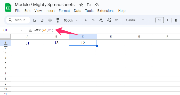
- Step 3: Click on the functions (fx) field, and enter the “=MOD(A1, B1)” formula.
- Step 4: It will return “12” as the output in the C1 cell.
Bonus: Do you know that you can now even insert emojis and special characters in Google Sheets to increase the aesthetic appeal? Don’t forget to check out my 2023 guide on how to insert emojis in Google Sheets the easy way!
Tracking Recurring Events Or Patterns
We often need the grids (pros call them the Zebra lines) when we want to take a printout of our spreadsheet. However, it is better if we assign colors to alternating rows.
You can use the “MOD” function in this case to track and highlight even or odd rows. Let’s see how we can do it easily.
- Step 1: Launch Google Sheets and open the spreadsheet.
- Step 2: Click on the “Format” option from the header menu.
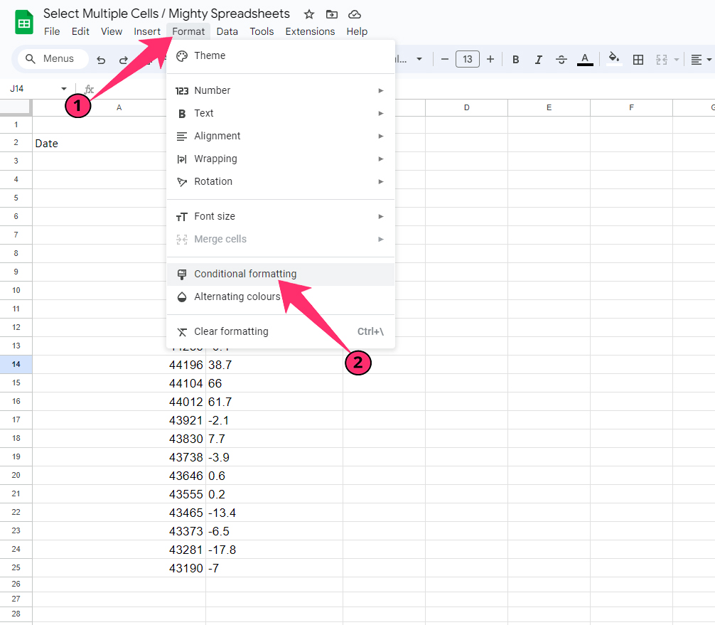
- Step 3: Click on the “Conditional Formatting” option, and a side widget will load.
- Step 4: From the header menu of the sidebar, navigate to the “Single Color” option.
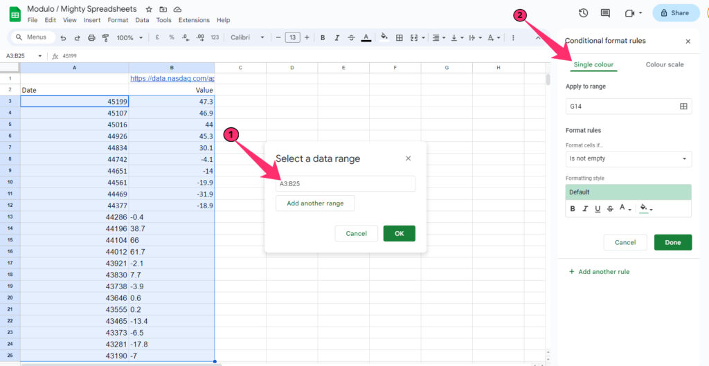
- Step 5: Define your cell range in the “<First cell>:<Last cell>” format in the blank field under the “Apply to range” header.
- Step 6: Click on the drop-down menu beneath the “Format cells if…” option.
- Step 7: Click on the “Custom Formula Is” option.
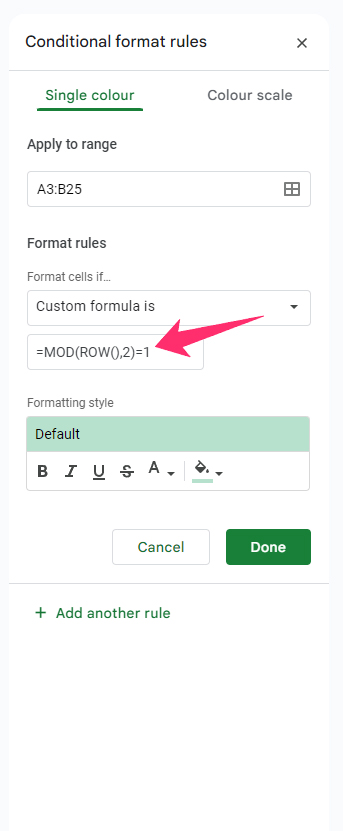
- Step 8: Now, enter the “=MOD(ROW(),2)=1” formula in the “Value or Formula” bar to highlight alternating rows starting from the first row.
- Step 9: To highlight the even-numbered rows, use the “=MOD(ROW(),2)=0” formula.
- Step 10: Select your color and other customizations in the “Formatting style” segment.
- Step 11: Click on the “Done” button, and the alternating rows will be highlighted.
There are other ways also available where you can track a particular pattern using the MOD function. However, it makes the formula complex and can even return an error if there is a zero or blank value in a cell.
Tips And Tricks For Working With Modulo In Google Sheets
There is no doubt that the modulo operator is a useful function in Google Sheets. However, it can also return an error output if we don’t use it right. So, let’s see how we can work with those errors and fix those!
Handling Errors And Zero Division
Let’s take a walk through the down-memory lane to our school days! When we divide something with 0, the result is undefined (you can call it a type of singularity, but not infinity).
So, if you use “0” as the divisor in the MOD function, it will return an “#DIV/0!” error that denotes the undefined output. But there is a workaround if we use the “IFERROR” formula with the MOD function.
Example: We have “17” as the dividend in the A1 cell and “0” as the divisor in the B1 cell. The output cell is C1, but we don’t want to get an error, as we are trying to divide a number by zero.
- Step 1: Launch Google Sheets and click on the output (C1) cell.
- Step 2: Click on the Function (fx) field.
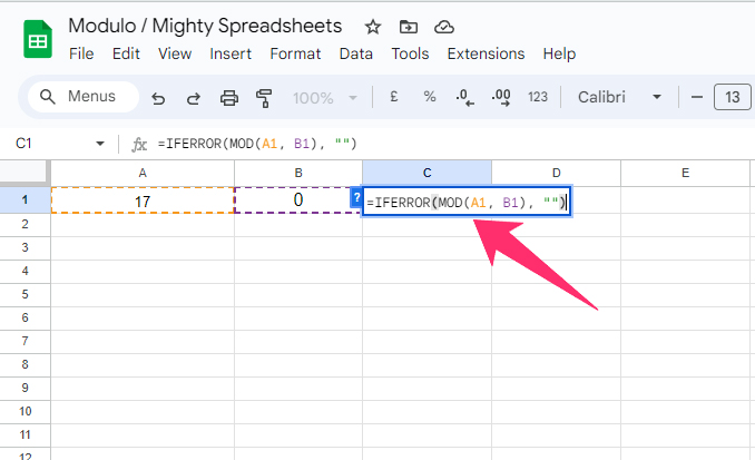
- Step 3: Now, enter the “=IFERROR(MOD(A2, B2), “”)” formula.
- Step 4: Hit the enter button, and it will return a blank value instead of the “#DIV/0!” error.
Note: If you are copying the formula and pasting it to other cells but still want to use the same reference cells, you need to use the absolute references in the formula.
So, instead of referring to the A1 cell, you need to refer to it as $A$1 cell. You can then copy the formula, and it will not automatically change the reference.
Modulo And Negative Numbers
Besides the positive integers, you can also use negative numbers in the MOD function in Google Sheets. And it will also give the output even if it is a negative number. Let’s understand with an example.
Let’s say we have -36 in the A1 cell and -7 in the B1 cell, and we want the remainder in the C1 cell.
- Step 1: Launch Google Sheets and click on the output (C1) cell.
- Step 2: Click on the “Function” (fx) field.
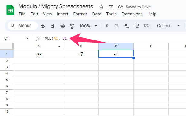
- Step 3: Out the “=MOD(A1, B1)” formula and hit the enter button.
- Step 4: It will return -1 as the output (remainder) in the C1 cell.
Please note that this function only works with numeric values (both positive and negative). So, if you are referring to a cell in this function, make sure that the cell must have a numerical value. Referring to a cell that has texts or alphanumeric will return an error.
Bonus: If you are using GS with your team for a collab project, it is necessary to check the editing history of your spreadsheet to find the latest changes. And to do that the right way, follow my comprehensive guide on how to see edit history in Google Sheets.
Testing Modulo Calculations With Other Functions
As I’ve said earlier, you can also use the modulo operator with other functions in Google Sheets. The prime examples are sure the “AND,” “IF,” “OR,” and “IFERROR” functions. However, you can use the MOD function with other functions as well.
Let’s try to convert seconds in the “HH:MM:SS” format using the MOD function. We will also be using the “TRUNC” and the “TEXT” formula.
The main formula is “=TRUNC(<reference cell>/3600)&TEXT(MOD(<reference cell>/86400,1), “:MM:SS”)” that we will be using here. And we have the 15,500 seconds in the A1 cell that we want to convert into the “HH:MM:SS” format in the B1 cell. Let’s check out the steps.
- Step 1: Launch Google Sheets and open your spreadsheet.
- Step 2: Click on the output cell (Here, it is B1).
- Step 3: Click on the function (fx) field.
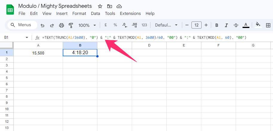
- Step 4: Put the “
=TEXT(TRUNC(A1/3600), "0") & ":" & TEXT(MOD(A1, 3600)/60, "00") & ":" & TEXT(MOD(A1, 60), "00")” formula and hit the enter button. - Step 5: It will return “4:18:20” in the B1 cell.
Here, we have first divided the seconds by 3,600 because there are 3,600 seconds in an hour, which is required for minutes calculation as a remainder.
And then we have also divided the seconds with 86,400 as there are 86,400 seconds in a day, and it is required to calculate hours as a remainder.
Conclusion
If you are using the modulo operator for any simple calculation, it is better to use the numeric values inside the formula rather than using a reference cell. Even if you are using a reference cell in the formula, make sure it has a numeric value.
You also need to remember that using “0” as the divisor in the MOD function will return an error. So, if you are using this function with some other function, make sure that you are not using “0” in the function.
However, you can surely use the IFERROR function along with the MOD function to ensure it returns a blank field rather than the “#DIV/0!” error.
FAQs
How do I get only the remainder in Google Sheets?
You can use the “MOD” function, also known as the modulo operator, in Google Sheets to get only the remainders. Use the “=MOD(<Dividend>, <Divisor>)” formula in the output cell, and you’ll get only the remainders.
You can either directly insert the numeric values or can also reference cells in the formula.
Can Modulo be used to create dynamic formulas in Google Sheets?
Yes, you can definitely use the modulo operator with other functions to make a dynamic and complex formula. For logical reasoning, the MOD function works well with the “IF,” “And,” and “Or” functions. You can also use it with other conditional formulas, such as the “IFERROR.”
Is there a limit to the size of the numbers I can use in Modulo calculations?
No, there is no such upper limit on the size or value of the dividend or the divisor in the modulo operation in Google Sheets. However, zero cannot be used as the divisor in the formula, as it will return an error.