How To Make Text Vertical In Google Sheets? (A Step-By-Step Guide For Beginners)

We all need to include vertical texts in our spreadsheet while we work with a large dataset or if we need to increase the aesthetic appeal. But do you know how to make text vertical in Google Sheets? Let’s find out with the Mighty Spreadsheets! 

To make a text vertical, select the cell first and then click on the “Text Rotation” option from the toolbar. Choose among “Stack Vertically,” “Rotate Up,” and “Rotate Down,” and it will arrange accordingly. You can also tilt the text from a certain angle while using the “Custom Angle” option.

You can also do the same thing from the “Format” option in the header menu. Otherwise, you can also use the REGEXREPLACE function to stack the text vertically. Let’s see all the methods in detail.

How To Make Text Vertical In Google Sheets?

We often need vertical text in Google Sheets, mainly in the header, to denote a particular type of data. Many use this for decorative purposes as well. So, we decided to make a comprehensive guide to help newbies in GS.

Step-By-Step Instructions For Rotate Text 90 Degrees In Google Sheets (In Mobile App Also)

You can easily stack texts vertically in any spreadsheet tool. But it is also true that most people find stacked-up texts challenging to read. So, you need to know how to rotate text in Google Sheets. It is easy, though!

• Step 1: Launch the spreadsheet in Google Sheets.
• Step 2: Click on the cell where you want to rotate the text 90° to select it.
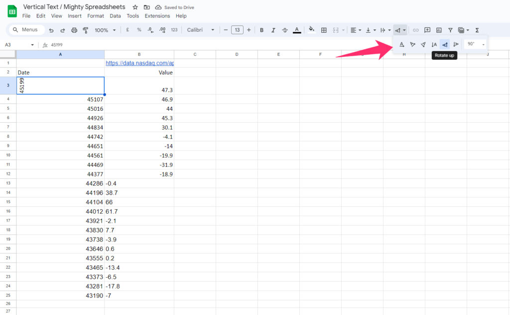
• Step 3: Navigate to the toolbar and click on the “Text Direction” option (“A” with an arrow beneath it).

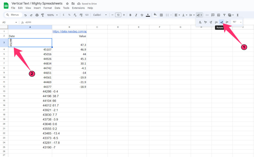
• Step 4: Click on the “Rotate Up” option (Sidewise “A” with an arrow pointing upwards).
• Step 5: Your text is not vertical. But you need to wrap the text if the content is lengthy.
• Step 6: Alternatively, click on the cell again to rotate the text inversely (-90°).
• Step 7: Click on the “Text Direction” button again on the toolbar.

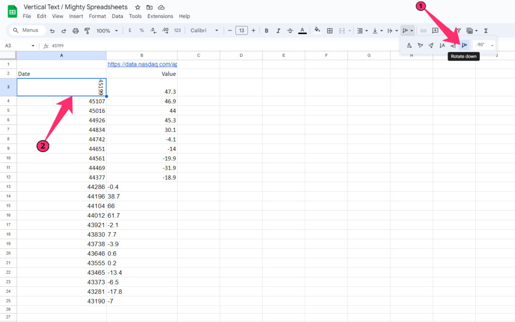
• Step 8: This time, click on the “Rotate Down” option (Sidewise “A” with an arrow pointing downwards).

Both the text directions also work in merged cells, as you may need to use it to make a title row that has further branches with multiple rows. Besides, you can do the same way in the app as well.

Bonus: Do you know how useful the “IF” formula is in any spreadsheet app? Check out my 2023 guide on using the “IF” formula in Google Sheets to know more!

How To Use Rotate Text In Google Sheets Option To Customize Text Orientation?

You must have already understood how to use google sheets to rotate text 90 degrees in your spreadsheet. However, this amazing tool also gives you the option to have different orientations, even in vertical texts. Let’s see how to do that!

• Step 1: Launch Google Sheets and click on the cell in which you want to change the orientation.
• Step 2: Go to the toolbar and click on the “Text Rotation” button.
• Step 3: It will show five orientation styles besides the default (left to right) one: “Tilt Up,” “Tilt Down,” “Stack Vertically,” “Rotate Up,” and “Rotate Down.”

• Step 4: Click on your preferred style, and the text you have selected will automatically change its orientation.
• Step 5: Alternatively, you can also find a small drop-down menu right beside the orientation symbols.
• Step 6: Choose any orientation between 90° and -90°, and the text will change the orientation.

Besides changing the orientation, you can also customize the vertical alignment and the horizontal alignment in your cell as well. You can find the options on the left side of the “Text Rotation” option.

How To Apply Vertical Text In Google Sheets To A Specific Cell, Range Of Cells, And Merged Cells?

I’ve already shown you all the ways to make vertical text in Google Sheets. But besides applying to a single cell, you can make the text vertical by default in multiple cells, even on a merged cell. Let’s see how we can do that!

• Step 1: Open the spreadsheet in Google Sheets.
• Step 2: Click on the first cell of your desired cell range.
• Step 3: Drag the cursor diagonally to select the range (Alternatively, you can enter the entire cell range in the “<First cell>:<Last cell>” format in the name box.

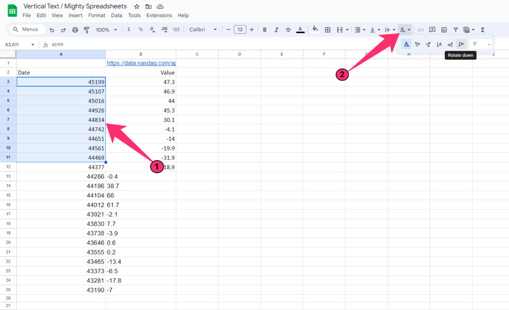
• Step 4: Click on the “Text Rotation” icon on the toolbar.
• Step 5: Click on the “Rotate Up” or “Rotate Down” option according to your preference.
• Step 6: To do the same on a merged cell, start by selecting all the cells that you want to merge.
• Step 7: Click on the “Format” option from the menu and click “Merge Cells.”

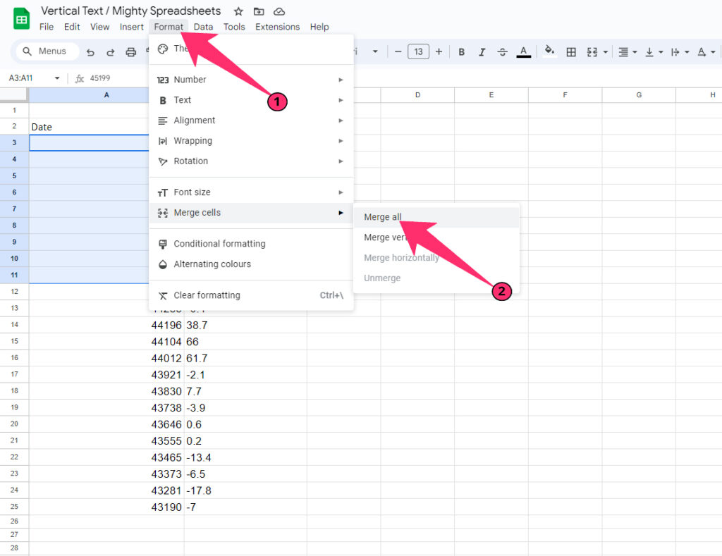
• Step 8: Click on the “Merge All” option and then click on the “Text Rotation” button again.
• Step 9: Select your preferred orientation, and the content of the merged cell will display vertically.

Not just changing the orientation, you can now also insert emojis and special characters in GS. To know more, check out my detailed guide on inserting emojis in Google Sheets the easy way!

How To Make Text Vertical In Google Sheets?

We often need multiple revisions before we achieve the perfect stylization on our spreadsheet. And we need frequent edits as well. So, here goes our attempt to answer you if you don’t know how to make and edit text verticals in Google Sheets.

Step-By-Step Instructions For Changing The Text Direction To Vertical In Google Sheets

Before you start creating vertical text in Google Sheets, you need to know how many variants of vertical text this tool allows. There are three different vertical orientation styles available.

“Stack Vertically” is the first option, where each alphabet of a word will be displayed right beneath the previous alphabet. The second option is “Rotate Up,” where the entire word changes its orientation while each alphabet leans sideways, pointing on the right side.

“Rotate Down” is the third option, where each alphabet will tilt sideways, pointing on the left side. And you can easily shift between three orientation styles.

• Step 1: Click on the cell or select the range of cells which you need to edit.
• Step 2: Once selected, click on the “Format” tab from the header menu.
• Step 3: Now, hover your cursor over the “Rotation,” and a new menu will appear on the side.

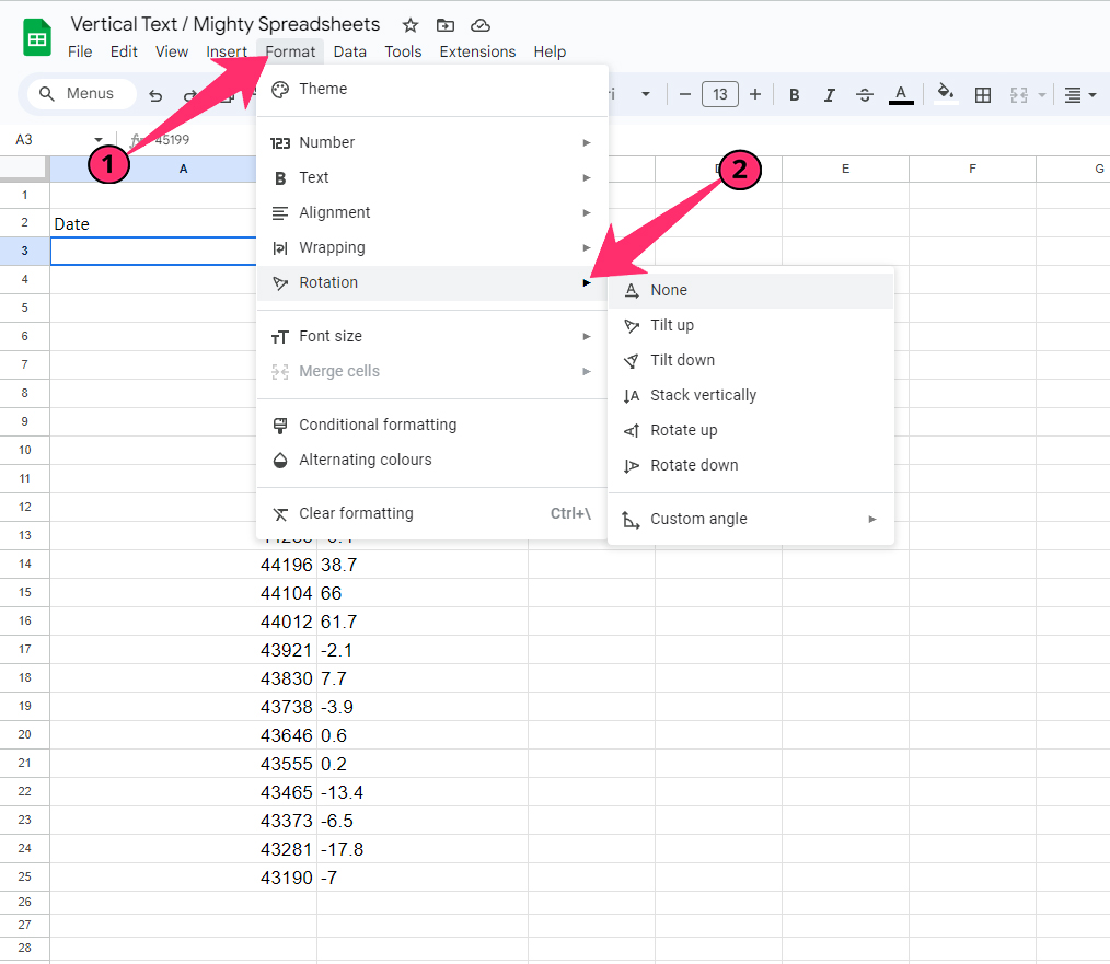
• Step 4: Click on the desired orientation style among “Stack Vertically,” “Rotate Up,” and “Rotate Down.”
• Step 5: You can now see that your text has the desired vertical orientation.

If you don’t want to display your text exactly in the upright or downright orientation, you can even imply some angles to it. To do that, click on “Format” followed by “Rotation.” Now, hover over “Custom Angle” and choose the desired angle from the list. 

How To Adjust The Text Alignment And Formatting For Vertical Text?

You must have already figured out how to turn text sideways in Google Sheets using the “Rotation” option. But besides the orientation, you can also change both the vertical and horizontal alignment, even on your vertical text.

• Step 1: Launch Google Sheets and open your spreadsheet.
• Step 2: Click on the cell or select the entire cell range that has vertical texts.
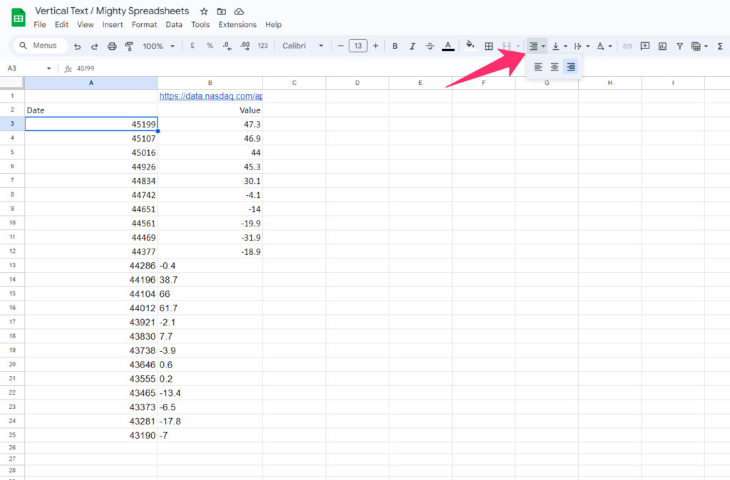
• Step 3: Navigate to the toolbar and click on the “Horizontal Align” option.
• Step 4: From the drop-down menu, choose your vertical alignment among “Center,” “Left,” and “Right.”

• Step 5: Now click on the “Vertical Align” option on the toolbar (right beside the “Horizontal Align” button).

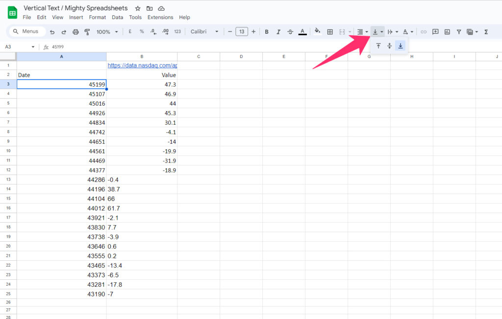
• Step 6: Select your desired orientation among “Top,” “Middle,” and “Bottom.”
• Step 7: The alignment (both vertically and horizontally) of your vertical text is now changed.

There is no way to change the direction of the text on a spreadsheet, as it is implied by default as left to right. And if you want to change it from right to left, you need to do it from the actual settings.

• Step 1: Navigate to the home screen on your Google Sheets account.
• Step 2: Click on the “Menu” option (Three horizontal lines -stacked) located in the top-left corner.

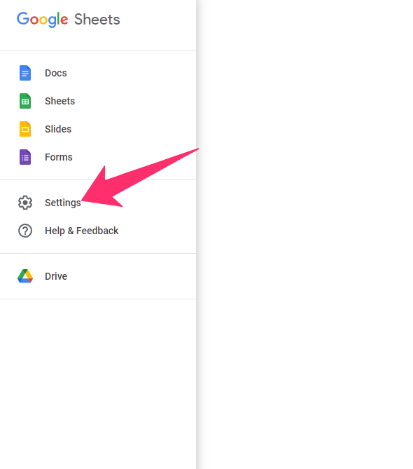
• Step 3: From the menu, click on the “Settings” option.
• Step 4: Tick the box beside the “Always show right-to-left controls” option.

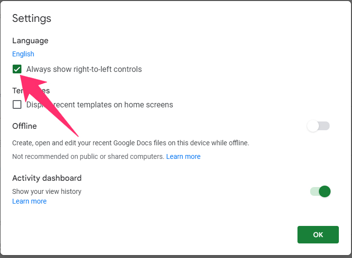
• Step 5: Click “OK” and refresh your Google Sheets.
• Step 6: Now, open the spreadsheet, and you’ll get the “Right to left” option in the “Cell Direction” menu as well.

If you are using vertical text in any row header, you need to adjust the height of the header accordingly to fit the entire text in the visible space. To do that the easy way, follow my latest guide on adjusting row height in Google Sheets.

How To Turn Text Sideways In Google Sheets?

You have already grasped how to make text in Google Sheets vertical. But there are two ways to make the text turn sideways. You can point it leftwards where the alphabets go from bottom to top. And you can also point it rightwards where the alphabets arrange from top to bottom.

And it is easy to do both sidewise orientations. Check out the steps.

• Step 1: Launch Google Sheets and open your spreadsheet.
• Step 2: Click on the cell where you need the sidewise texts.
• Step 3: Click on the “Text Rotation” button on the toolbar.

• Step 4: Now, click on the “Rotate Up” button if you want to make your text face on the left.
• Step 5: Choose “Rotate Down” if you need the text to face rightwards.

There is no way to change the direction of the text if you make it sideways. If you choose the “Rotate Up” option, the text will start from the bottom and move upwards. And if you choose “Rotate Down,” the text will start from the top and move to the bottom.

How To Edit And Format Google Sheets Vertical Text?

Once you know how to rotate text in Google Sheets, you can now start practicing some more customization options. Yes, it is possible to incorporate various customizations, even on vertical texts. Let’s see what we can do about that!

How To Change The Font, Size, Color, And Alignment Of Vertical Text?

You can easily alter the alignment of vertical text, both horizontally and vertically. And we have already discussed how to do that! Now, let’s see how we can change the font, font size, and color of the text.

Changing Font Style:

• Step 1: Click on the cell where you have the vertical text.
• Step 2: Navigate to the toolbar and click on the “Font” option.

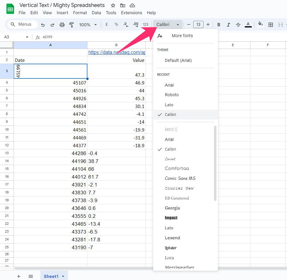
• Step 3: Select the font style from the list (the default is Arial).

Changing Font Size:

• Step 1: Click on the cell and navigate to the toolbar.
• Step 2: Click on the “+” or “-” signs beside the “Font Size” to increase and decrease the font size.

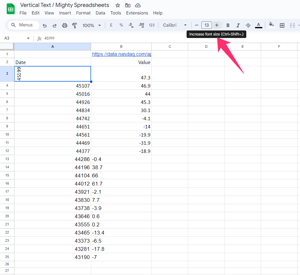
• Step 3: Alternatively, double-click on the “Font Size,” and a list of options will appear.
• Step 4: Choose your desired font size (6 to 36) from that list.

Changing Text Color:

• Step 1: Click on the cell that you want to modify.
• Step 2: Go to the toolbar and click on the “text Color” option (“A” icon with a small colored block beneath it).

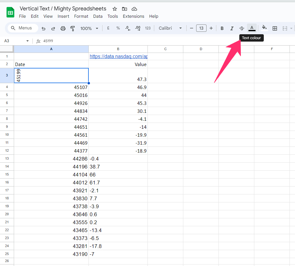
• Step 3: Select your desired color from the palette.

As you can see, the default font in Google Sheets is Arial. However, you can make almost any font a default. To do that, check out my detailed guide on changing the default font in Google Sheets.

How To Change Text Direction In Google Sheets?

There are three ways you can arrange vertical text in Google Sheets. You can stack one alphabet over another; you can make the text sideways on your right or can make it sideways on your left. Let’s see how we can assign these directions.

• Step 1: Launch Google Sheets and open your spreadsheet.
• Step 2: Click on the text in which you want to make the text vertical.
• Step 3: Navigate to the toolbar and click on the “Text Rotation” button.
• Step 4: Click on the third option to stack the text vertically.
• Step 5: If you want to start your vertical text from bottom to top while the alphabets face the left side, click on the “Rotate Up” option.

• Step 6: To do the exact opposite things where alphabets will face the right side, click on the “Rotate Down” button.

Besides just top to bottom or bottom-to-top arrangements, you can also arrange diagonal text directions. You can even assign a degree of tilt to any text in Google Sheets.

Tips For Creating Effective Vertical Text In Google Sheets

After you know the ways to change text direction in Google Sheets, you then need to properly optimize it to make it look good whenever you apply it to your spreadsheet. So, let’s see how we can organize and optimize our vertical texts!

Best Practices For Creating Clear And Legible Vertical Text

Start by restraining yourself from using flashy font style and color, as it can seriously disturb the overall aesthetics rather than improve it. 

You should also try not to make the vertical text too big by increasing the font size. Besides, it is also not recommended to use special symbols in vertical texts as it will be hard for users to understand.

If you have a lengthy text placed vertically, not all the text will be displayed until you make some adjustments. Let’s see how we can do that.

• Step 1: Launch Google Sheets and click on the cell where you have the vertical text.
• Step 2: You can also choose the entire range if you have vertical texts in more than one cell.
• Step 3: Click on the “Format” option from the header menu.

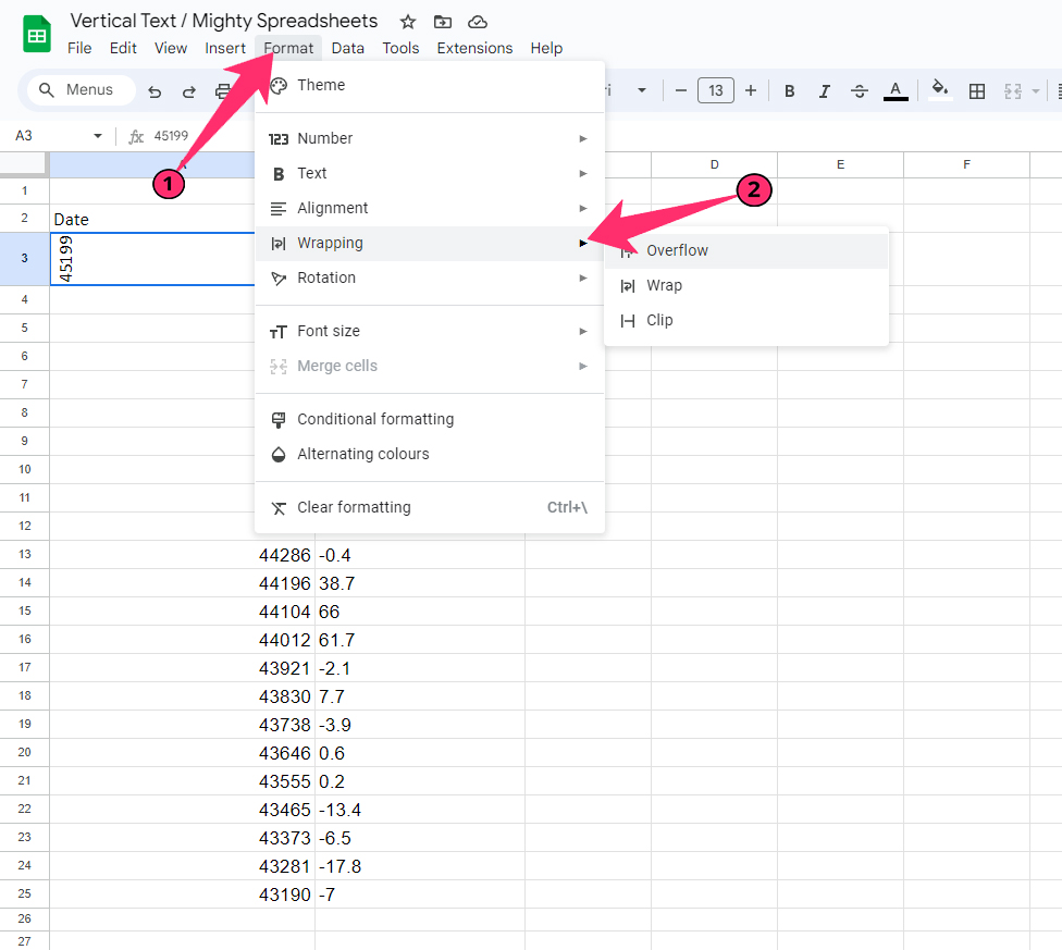
• Step 4: Hover your cursor over the “Wrapping” option, and a side menu will load.
• Step 5: Click on the “Overflow” option, and your entire vertical text will start displaying on the cell.

If you want to select any other arrangements, then you can adjust the row height manually. Follow the steps to do that!

• Step 1: Select the cell that has the vertical text and enable the “Overflow” wrapping.
• Step 2: Now, hover your cursor over the border of the row header label.
• Step 3: Once your cursor changes into an arrowhead, double-click on it.
• Step 4: It will auto-adjust the row height according to the text inside it.

Bonus: Do you know that you and your teammates can now simultaneously work on the same spreadsheet? Check out my 2023 guide to share and collaborate in Google Sheets to know more!

Suggestions For Organizing And Formatting Vertical Text To Make It Easy To Read

If you have too many rows that have vertical texts, it will not be possible to adjust the row height for each one. In that case, it is better to use a fixed row height. The steps are pretty easy!

• Step 1: Open your spreadsheet in Google Sheets.
• Step 2: Navigate to the row where you have vertical texts and go to the header label.
• Step 3: Right-click on the header label, and a contextual menu will appear.
• Step 4: Click on the “Resize the row” option from the menu, and a popup window will appear.
• Step 5: Tick the “Fit to data” option and then click on the “OK” button.
• Step 6: Your rows will now automatically adjust according to the data length.

If you have any specific design template for the vertical texts, you can now also adjust the row height accordingly. And to do that, follow the above steps but choose the “Specify row height” option rather than the “Fit to data” option.

You can then manually enter the height of the row (in pixels), and it will automatically adjust.

Best Practices For Using Vertical Text In Charts, Tables, And Other Types Of Data

You have already understood how to make text vertical in Google Sheets when you are using a simple spreadsheet. But you can even integrate vertical and diagonal texts in different charts and tables on GS.

Make Text Diagonal In Google Sheets

We often need to make the text tilt a little to go aesthetically well with the chart we have on the spreadsheet. And with the “Text Rotation” option, you can now align the text at different angles. Let’s see how we can do it easily!

• Step 1: Launch Google Sheets and click on the cell that has vertical text to select it.
• Step 2: Click on the “Format” option from the header menu.
• Step 3: On the menu, hover your mouse over the “Rotation” option, and a side menu will appear.
• Step 4: Click on the “b” option if you want to make the text appear diagonally in the top-right direction.

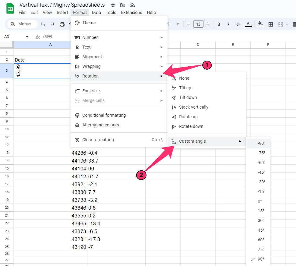
• Step 5: Select the “Tilt Down” option if you want to make it diagonally in the down-right direction.
• Step 6: To choose a different angle of tilt, hover your mouse over the “Custom Angle” option.
• Step 7: Click on the desired degree of angle (From +90° to +90°) of your tilted text.

You can also alternatively make a text box and tilt it at any angle before integrating it into your spreadsheet. To do that, click on the “Insert” option from the header menu and then click on the “Drawing” option.

Once the drawing window appears, click on the “Text Box” option from the header menu. Now, tilt it in any direction while holding the upper marker of the text box.

Advanced Techniques For Vertical Text In Google Sheets

It is easy to know how to make text vertical in Google Sheets with the help of the “Text Rotation” option. But stacking up alphabets can also be done in other ways on GS.

Creating Unique Vertical Text Effect In Google Sheets Using Custom Formula

Let’s say I have a text in the A1 cell, and I want to make it vertical (stacked up vertically) in the B1 cell. We will be using the “REGEXREPLACE” function here. Let’s check out the steps.

• Step 1: Launch your spreadsheet on Google Sheets and click on the output cell (Here it is B1).
• Step 2: Click on the “Function” (fx) field.
• Step 3: Put the “=REGEXREPLACE(A1,"(.)","$1"&CHAR(10))” formula and hit the enter button.
• Step 4: Your text will now stack up vertically in the B1 cell.
• Step 5: Alternatively, you can directly include a text in the formula rather than referring to an input cell.
• Step 6: To do that, enter the “=REGEXREPLACE(“<text>”,”(.)”,”$1″&CHAR(10))” formula.

You need to remember that this formula will only stack the alphabets of the text vertically, where the alphabets will be placed on top of one another. However, you can’t do it for the sideways text using a formula.

Final Note

It is easy to know how to make text vertical in Google Sheets, although we have included various methods to do that. But if you want the easiest route, it is better to access the “Text Rotation” option on the toolbar, which gives you various rotation options, including tilts.

However, you need to keep the vertical text short, especially if you are using “Text Wrapping” to display the entire text in a cell. Otherwise, your row height will be too much, and it will surely disturb the overall aesthetics. The trick is to make it look simple yet easily readable!

FAQs

How Do I Change Text From Horizontal To Vertical In Google Sheets?

Click on the input cell to select it, and then click on the “Text Rotation” option on the toolbar. You can now use the “Stack Vertically,” “Rotate Up,” and “Rotate Down” options to rotate the text from a horizontal to a vertical direction, depending on your requirement.

How Do I Flip Data From Horizontal To Vertical In Google Sheets?

If you are creating a chart on Google Sheets where you need to flip the data from the horizontal to the vertical direction, you can do it with the “Chart Editor” option.

Double-click on the chart and click on the “Setup” button on the right. Now, click on the “Switch rows/columns” option to flip the entire data.

Is Vertical Text Useful In Charts And Tables?

Yes, vertical text is extremely useful in charts and integrated tables in Google Sheets. If any element of your chart has a y-axis direction, you can then label it with vertical text.

You can also do it on a table if you want to label the Y-axis of any embedded table in a spreadsheet.

Can I Use Custom Formulas Or Scripts To Create Unique Vertical Text Effects In Google Sheets?

Yes, you can use the REGEXREPLACE function to create unique stacked vertical text in Google Sheets. And to do that, use the “=REGEXREPLACE(<input cell>,”(.)”,”$1″&CHAR(10))” or the “=REGEXREPLACE(“<text>”,”(.)”,”$1″&CHAR(10))” formula.