How To Calculate Age In Google Sheets? Steps EXPLAINED!

If you are keeping any personal record, such as employee data, you may need to calculate the age from the date of birth. And it is possible to do so on spreadsheets. But do you know how to calculate age in Google Sheets the easy way?

To get the age just in years format, you can use the “YEARFRAC” function along with the “INT” function. It is a simple formula. However, if you want to get the recent age in years, months, and days format, you need to use the “DATEDIF” formula.

But you also need to understand your default date format in Google Sheets. Otherwise, you may get an error output. So, let’s see how to calculate the age and how to understand the date formats to use in the age calculation.

Understanding Date Formats In Google Sheets

Before you start the process of calculating age in Google Sheets, you need to know about the different date formats available on Google Sheets. Let’s know in detail!

Date Format Options Available In Google Sheets

We all know that Microsoft Excel understands all the date formats, including the text formats, such as 31^st July 2023. But Google Sheets only understands dates in an integer value, such as 31/07/2023.

However, depending on the region you have specified in Google Sheets, your format will appear differently, such as “DD/MM/YYYY” and “MM/DD/YYYY.” It is possible to change between these formats.

• Step 1: Launch Google Sheets and open a spreadsheet.
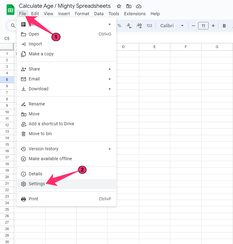
• Step 2: Click on the “File” button from the header menu.
• Step 3: Now, click on the “Settings” option.

• Step 4: Navigate to the “General” tab from the header selection options.
• Step 5: Click on the drop-down list below the “Locale” option.

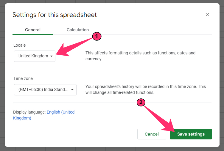
• Step 6: Select your region from the list.
• Step 7: Click on the “Save And Reload” button in the bottom-right corner.

Some of the available date formats (depending on region) in Google Sheets that I found are as follows.

• United States: MM/DD/YYYY
• United Kingdom: DD/MM/YYYY
• Canada: YYYY-MM-DD
• Australia: D/MM/YYYY
• Germany: DD.MM.YYYY

To check what is the date format in your current settings, follow the method mentioned below.

• Step 1: Launch Google Sheets and open a spreadsheet.
• Step 2: Click on the “Format” option from the header menu.
• Step 3: On the drop-down menu, hover your mouse over the “Number” option, and a side menu will appear.

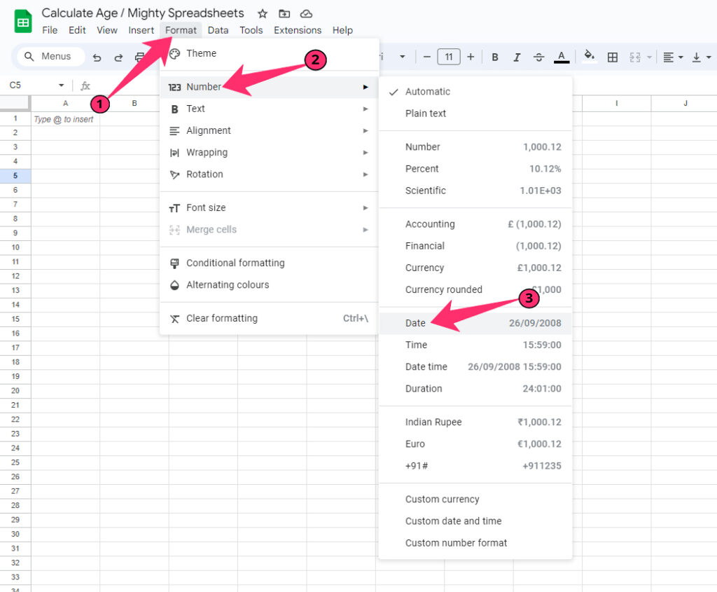
• Step 4: Find the current date format beside the “Date” option.

Bonus: At times, you may need to insert a page break in your spreadsheet to differentiate between two data sets. To do that the right way, follow my comprehensive guide on inserting page breaks in Google Sheets.

Converting Text To Date Format In Google Sheets

If you have a date written in text formats, such as 9^th August 1990 or 9 Aug 1990, you can also convert that to the default date format in Google Sheets.

And there are two methods available to do that. The first one is by using the in-built format option. And the second one is by getting an add-on, such as Power Tools by Ablebits.

Let’s say we have “9^th August 1990” written on the A1 cell. And we want to convert that to the default date format. Let’s start with the easy one.

• Step 1: Click on the A1 cell where you have the date to select it.
• Step 2: Click on the “Format” option from the header menu.
• Step 3: Hover your mouse over the “Number” option.

• Step 4: On the side-loaded menu, click on the “Date” option.
• Step 5: You can now see “09/08/1990” as the output.

I got this format as my default regional setting is “United Kingdom.” You will get the default date format depending on your respective country.

Using Third-Party Add-Ons To Convert Text To Date Format

The second method we will be talking about is the usage of third-party tools for converting text to date format. This is especially helpful if you want to convert a large set of data but don’t want to do it manually (as it will take a huge amount of time).

There are many add-ons available on the Google Workspace Marketplace that can do that. But my personal favorite is surely Power Tools by Ablebits. Now, let’s check out the steps!

• Step 1: Launch Google Sheets and open a blank spreadsheet.
• Step 2: Click on the “Extension” option from the main menu.

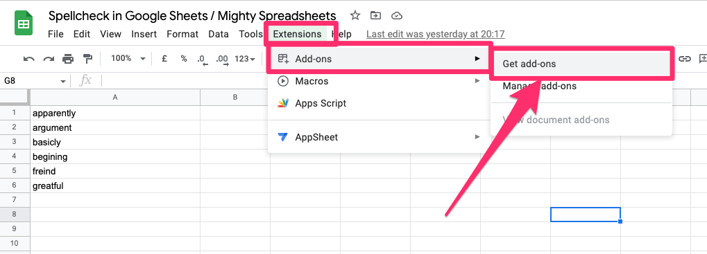
• Step 3: Hover your mouse over the “Add-ons” option and click on “Get add-ons.”
• Step 4: Now, click on the search bar in the newly opened window.
• Step 5: Type “Power Tools” in the designated search field and hit enter.
• Step 6: Click on the first result and then on the “Install” button.

• Step 7: Allow all the necessary permissions to complete installation.
• Step 8: Reload Google Sheets and click on the “Extension” option again.
• Step 9: Click on the “Power Tools” option, and a side-loaded widget will appear.
• Step 10: Select the reference cell and navigate to the Power Tools widget.
• Step 11: Click on the “Convert” radio button from the main header menu.
• Step 12: Click on the “Convert date formats and number signs” option to expand the list.
• Step 13: Select the “Convert text to dates” option.
• Step 14: Click on the “Run” button.
• Step 15: You can now see your text is converted to the default date format on the same cell.

Fun Fact: Do you know that you can even insert emojis in your spreadsheet? Check out my latest guide on inserting emojis and special symbols in Google Sheets to know in detail.

How To Calculate Age In Google Sheets?

Google Sheets is one of the most versatile Google Workspace tools that comes with several unique features. Besides, it is as competent as the age-old Microsoft Excel, as you can get identical functions on both platforms.

However, it is easy to calculate age in Google Sheets! There are two functions available: DATEDIF and YEARFRAC. Among these two, the first one is way more versatile. Now, let’s check these two functions in detail!

Calculating Age With The “INT” Function

This method will work if you need just the years while calculating age in Google Sheets. You can use the INT function and define both the start and the end date to do it.

The syntax we will be using here is “=INT((<Start Date>()-<End Date)/365)”

Here, we will be using the “09/08/1990” as the start date (date of birth) and the “TODAY” function as the end date. And we will divide it with 365 to get the year count. Now, let’s check out the steps!

• Step 1: Launch Google Sheets and open the spreadsheet where you want to calculate the age.
• Step 2: Click on the output cell (here, it is B1).
• Step 3: Click on the formula (fx) field.

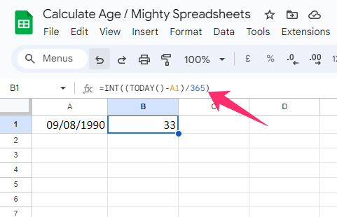
• Step 4: Enter the “=INT((TODAY()-A1)/365)” formula.
• Step 5: Hit the enter button, and you’ll get “33” as the output in the B1 cell.

Note 1: It will be a whole number. So, if the output is in decimals, it will take the next whole number. In this case, the actual elapsed year is 32, but we got 33 as the output, as this is the next whole number.

Note 2: Here, in this formula, we have not accounted for the leap years, as it will hardly make any difference unless the start and the end are too high. And that’s why we have used 365 to divide in this formula.

Calculating Age With The “DATEDIF” Function

I’ve previously said that the DATEDIF (which defines the difference between dates) function is the most versatile one for calculating age in Google Sheets. Let’s know about the syntax first.

Syntax: “=DATEDIF(<Starting Date>,<Ending Date>,<Unit>)”

The “Starting Date” on this syntax is the date from which you want to start the age calculation, thus the actual birthdate. And the “Ending Date” is the date you want to calculate the age. Mostly we will be using the current (today’s) date for this one.

Now, there are six types of unit parameters you can use on this syntax, which are “Y,” “M,” “D,” “YM,” “YD,” and “MD.” Let’s know about each one.

• “Y” (Stands for “Year”): It is the total number of completed years between the start and the end date.
• “M” (Stands for “Month”): This parameter will calculate the total number of completed months between given dates.
• “D” (Stands for “Day”): Now, this one will calculate the total number of completed days between dates.
• “YM”: This will calculate the total number of months remaining after completed years. And this value can’t go beyond 11 (because 12 will complete a year).
• “YD”: This will calculate the total days remaining after the completed years. However, this can’t exceed 364 (because 365 will complete a year).
• “MD”: It is used for calculating the total number of days remaining under completed months.

You can only use a single parameter in a single syntax. However, you can also combine many parameters to make a complex formula. You can even use the ARRAY functions with these parameters as well.

Calculating Individually With Each Parameter (Simple Method)

We will be calculating year, month, and day individually first (fully elapsed) with this method. Let’s say we have the “09/08/1990” date in the A1 cell. And we will be calculating the total number of completed years in the B1 cell, total months in C1, and total days in D1.

We will also be using the “TODAY” function with the “DATEDIF” function to do it. Here are the steps.

• Step 1: Click on the “B1” cell.
• Step 2: Click on the formula field (fx) and enter the “=DATEDIF(A1, TODAY(), “Y”)” formula.

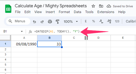
• Step 3: Hit the enter button, and it will return “32” in the B1 cell.
• Step 4: Now, click on the “C1” cell to get the month-wise output.
• Step 5: Click on the “fx” field and enter the “=DATEDIF(A1, TODAY(), "M")” formula.

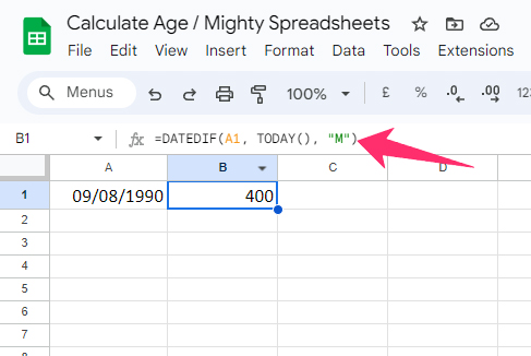
• Step 6: Hit enter, and it will return “400” in the C1 cell.
• Step 7: To get the day output this time, click on the D1 cell.
• Step 8: Use the fx field to enter the “=DATEDIF(A1, TODAY(), “D”)” formula.

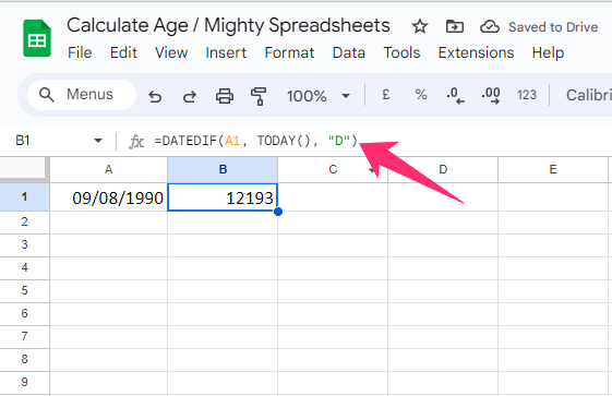
• Step 9: Hit enter, and it will return “12047” in the D1 cell.

Explanation: As of making this post on 4^th August 2023, the total number of years elapsed from 9^th August 1990 is 32, elapsed month is 395, and elapsed day is 12047.

If you have two separate dates in two separate cells, such as 09/08/1990 in A1 and 31/07/2023 in A2, you can also define just the cells to get the age till the given date.

And to do that, use the “=DATEDIF(A1,A2(), “Y”)” formula to get the output till the defined date.

Bonus: Do you know that “IF” is a superiorly versatile function? To know more, check out my latest guide on the “IF” function in Google Sheets.

Calculating Age Combining All Parameters (Complex Method)

We will now combine all the parameters to get a joined output where we want all the completed years, months, and days to be displayed together. And for that, we will be using the DATEDIF function along with the TODAY and & (to join) functions.

I’m taking the same example to demonstrate where I have the “09/08/1990” date in the A1 cell. We will now get the output in the B1 cell. Check out the steps!

• Step 1: Click on the B1 cell.
• Step 2: Click on the formula (fx) field.
• Step 3: Enter the “=DATEDIF(A1,TODAY(),”Y”)&” Years “&DATEDIF(A1,TODAY(),”YM”)&” Months & “& DATEDIF(A1,TODAY(),”MD”)&” Days”” formula.

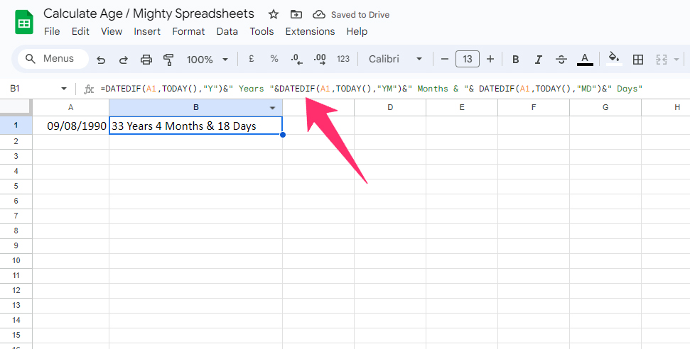
• Step 4: Hit the enter button, and you’ll get “32 Years 4 Month & 18 Days” as the output in the B1 cell.

Now, let’s say we have four different dates in A1 to A4 cells. The spreadsheet has 09/08/1990 in A1, 12/01/1990 in A2, 20/11/1995 in A3, and 10/12/1996 in A4.

I want to get the output with a single formula where all the ages will be calculated at once. And for that, we will be using the ARRAYFORMULA function along with the DATEDIF, TODAY, and & functions.

• Step 1: Click on the B1 cell (the first cell of your output range).
• Step 2: Click on the formula (fx) field.
• Step 4: Enter the “=ARRAYFORMULA(DATEDIF(A1:A4,TODAY(),”Y”)&” Years “&DATEDIF(A1:A4,TODAY(),”YM”)&” Months & “& DATEDIF(A1:A4,TODAY(),”MD”)&” Days”)” formula.

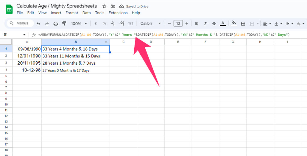
• Step 4: Press the enter button, and you’ll get “32 Years 11 Months & 25 Days” on the B1 cell, “33 Years 6 Months & 22 Days” on the B2 cell, “27 Years 8 Months & 14 Days” on B3 cell, and “26 Years 7 Months & 24 Days” on B4 cell.

Here, the ARRAYFORMULA function eliminates the need to use the formula each time for every output. And also to select the input value. This will directly select a range and deliver all output at once.

Bonus: Do you find it hard to clear all the formulas even after deleting the value from a cell? Then, check out my latest guide on how to clear content in Google Sheets to know more.

Calculating Age With The “YEARFRAC” Function

If you want to know just the exact year (fully elapsed) while calculating age in Google Sheets, you can also use the “YEARFRAC” function. It will give you direct results without any complications. You need to use the “YEARFRAC” function along with the “INT” function to get output.

The syntax we will be using here is “=INT(YEARFRAC(<Starting Date>,<Ending Date>())).”

Now, let’s say we have the same “09/08/1990” date in the A1 cell. And we want to get the exact age in years in the B1 cell. So, we will be using the “TODAY” function to assign current input.

• Step 1: Click on the B1 cell where you want to get the output.
• Step 2: Click on the formula (fx) field.
• Step 3: Enter the “=INT(YEARFRAC(A1,TODAY()))” formula.

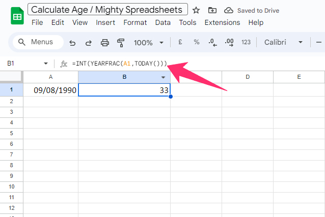
• Step 4: Hit the enter button, and you’ll get “32” as output in the B1 cell.

This time, we have the same four dates we have used in the “DATEDIF” formula. We have 09/08/1990 in A1, 12/01/1990 in A2, 20/11/1995 in A3, and 10/12/1996 in A4. Now, we will now try to get output at once.

• Step 1: Click on the B1 cell (the first cell of your output range).
• Step 2: Click on the formula (fx) field.
• Step 3: Enter the “=ARRAYFORMULA(INT(YEARFRAC(A1:A4,TODAY(),1)))” formula.

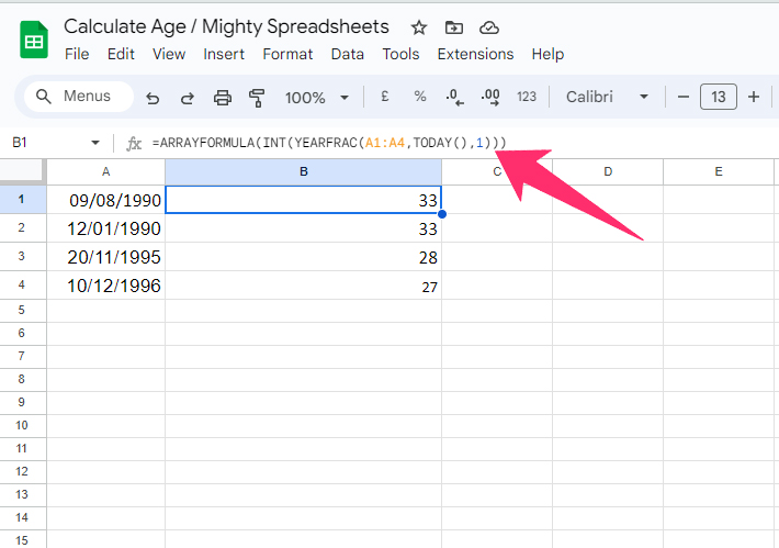
• Step 4: Hit the enter button, and you’ll get “32” in B1 cell, “33” in B2, “28” in B3, and “27” in B4 cell.

You can also make a slight modification in this formula if you want to make the input open-ended without specifying the end of the range. You can also define an entire column as the output for calculating age. 

We will be using the “IF” formula here. The steps are as follows.

• Step 1: Click on the B1 cell (the first cell of the output range).
• Step 2: Click on the formula (fx) field.
• Step 3: Enter the “=ARRAYFORMULA(IF(LEN(A1:A),(INT(YEARFRAC(A1:A,TODAY(),1))),))” formula.

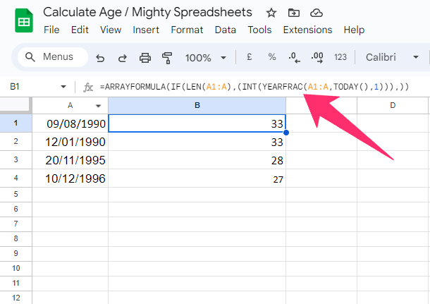
• Step 4: Hit the enter button to get the output.

Bonus: Do you know that you can now refer to another spreadsheet in a formula in Google Sheets? Check out how to refer to a spreadsheet in Google Sheets to know more.

Conclusion

 If you want just the age in years, it is best to use the YEARFRAC formula, as it can deliver direct output without any complicated formula. However, if you need to know the exact age in text format for better understanding, you must use the DATEDIF function.

But first, you need to check and fix the date formula you are using. Otherwise, the formula you are using to calculate age in Google Sheets may not count as a valid input.

FAQs

What is the formula for calculating age?

You can use either between the “=DATEDIF(<Starting Date>,<Ending Date>,<Unit>)” and the “=INT(YEARFRAC(<Starting Date>,<Ending Date>()))” depending on your need in Google Sheets. You can also combine the ARRAYFORMULA function to broaden the input range. 

How can I convert text to date format in Google Sheets?

Select the cell and click on the “Format” option from the header menu. From the contextual menu, hover your mouse over the “Number” option to get a side-loaded menu. Click on the “Date” option to convert text to date format.

How do I handle scenarios with past and future dates when calculating age?

Both the “=DATEDIF(<Starting Date>,<Ending Date>,<Unit>)” and “=INT(YEARFRAC(<Starting Date>,<Ending Date>()))” formula in Google Sheets supports any date you want. However, you can use the “TODAY” function to count it till the current day.