We often need to extract particular substrings from a range or a specific cell to get more structured data. A real example will be to extract the phone number from a cell that contains both the company profile along with the contact details. You can now easily extract substrings in Google Sheets by using some simple tricks.
You can use the LEFT, RIGHT, and MID functions to extract a substring from a particular position of a string. Besides, you can combine them with FIND and LEN to get the substring after or before specific characters where the output will be specific character long. You can even use Regular Expressions to make your formula shorter and more organized.
It is possible to combine various functions in Google Sheets to extract defined data or a particular match. But to keep it simple, here we will be using only those functions that you can use with ease without any complex method. So, let’s get started!
- Using Built-In Functions To Extract Substrings
- Method 1: LEFT Function To Extract A Substring From The Beginning Of The Text
- Method 2: RIGHT Function To Extract A Substring From The End Of The Text
- Method 3: MID Function To Extract A Substring From The Middle Of The Text
- Method 4: Get The Substring Before Certain Text
- Method 5: Get The Substring After Certain Text
- Using Regular Expressions For Advanced Substring Extraction
- Some Interesting Examples You May Like
- Key Takeaway
Using Built-In Functions To Extract Substrings
Google Sheets itself has some functions which you can use to extract substrings you’re your spreadsheets. And there are five different ways to do that, depending on your requirement.
We are going from the easiest to the most complicated one!
Method 1: LEFT Function To Extract A Substring From The Beginning Of The Text
You can use the “LEFT” function to extract a particular substring from a particular position inside a cell. The core formula we will be using is: “=LEFT(<String identifier>,<length>)”
The “String Identifier” is the string from which you want to extract, such as a cell. You can use the cell number in this parameter. And the “Length” is till which character in that string (counted from the beginning) you want to extract the data.
Example: We have a “+91-033-24448080” phone number in the A1 cell. It contains the country code (+91) and the city code (033), along with the actual number in the last eight digits.
So now, we want to extract the country and city code from the phone number in the B1 cell. We will use the “LEFT” function, and the steps are as follows.
- Step 1: Open the spreadsheet and select the empty cell where you want your output (here it is B1).
- Step 2: Click on the Formula (fx) bar.
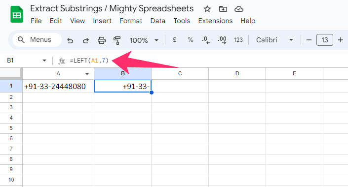
- Step 3: Enter the “=LEFT(A1,7)” formula (A1 cell is where the actual string is, and “7” is the character position till which we want to extract the substring).
- Step 4: Hit the enter button.
- Step 5: You’ll get “+91-033” (country and city code) in the B1 cell.
Note: Rather than manually entering the string identifier in the LEFT Function, you can just click on the cell you want to select after entering the “=LEFT(” part. It will automatically fetch the cell number in the formula.
You can now also apply the formula in the entire column in Google Spreadsheet. Check out my newest guide to know the steps and the easy ways to do it.
Method 2: RIGHT Function To Extract A Substring From The End Of The Text
Besides the “LEFT” function, you can also use the “RIGHT” function in Google Sheets to extract substrings. The core formula here will be “=RIGHT(<String identifier>,<length>).”
The string identifier is the cell or the range here from where you want to extract the substring. And the length is the number of characters you want to extract. But while “LEFT” counts it from the beginning, the “RIGHT” function counts it from the end, in reverse order.
Example: We will be using the same “+91-033-24448080” phone number with country code and city code. But this time, we want to extract the actual phone number (the last eight digits) from the string.
We have this phone number in the A1 cell and want to have the phone number as the output in the B1 cell. The steps to do that are as follows.
- Step 1: Select the cell where you want to get your output (Here it is B1).
- Step 2: Click on the Formula (fx) field.
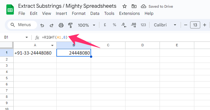
- Step 3: Enter the “=RIGHT(A1,8)” formula (A1 is the cell where we have the full number, and 8 is the number of digits we want to extract from the end).
- Step 4: Hit the enter button, and you’ll get “24448080” as the output in the B1 cell.
Note: If you have multiple strings in a column, such as a column full of phone numbers, you can use the formula in the first cell. And for the rest, you can simply drag it, and it will be automatically applied to every cell in that range.
Method 3: MID Function To Extract A Substring From The Middle Of The Text
While the “LEFT” and “RIGHT” functions help you to extract substrings from the beginning or the end of a string, the “MID” function lets you extract string from any position. It is also a bit more versatile than the previous two functions.
The main formula is “=MID(<String identifier>,<Start location>,<Length>)” in Google Sheets. Here, the “String identifier” is the cell or range from where you want to extract. The “Start location” is the position of the character from the beginning from where you want to start extracting.
And finally, the “Length” is the number of characters you want to extract from that string.
Example: We will be again using the same “+91-033-24448080” phone number in this case. But this time, we want to extract just the city code (033) from this string.
We have this number in the A1 cell and want to get the city code output in the B1 cell. Here are the steps.
- Step 1: Click on the empty output cell (It is B1 here).
- Step 2: Click on the formula (fx) field.
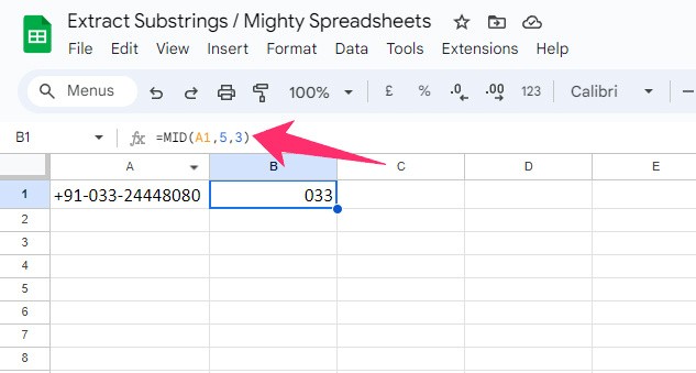
- Step 3: Enter the “=MID(A1,5,3)” formula (Starting location is 5 because the city code starts from the fifth position. And the length is 3 because the city code itself is 3 digits long).
- Step 4: Hit the enter button, and you’ll get “033” as the output in the B1 cell.
The “MID” formula gives you the option to pick up substrings from any position. But you need to count the empty spaces, special characters, and symbols, too, while selecting the starting location or the length.
Bonus: Grouping is necessary for Google Sheets, especially if you are working with a complex spreadsheet. Check out my latest guide on grouping and collapsing rows and columns in GS to know more!
Method 4: Get The Substring Before Certain Text
There is a way to extract a substring before certain text, symbol, or punctuation marks in Google Sheets. And you can easily do it by combining the “LEFT” function and the “FIND” function.
We will use the “=LEFT(<String identifier>,FIND(“<Text identifier>”,<String identifier>)-1)” formula in this case.
Here, the “String identifier” is the string or cell from where you want to extract your substring. The “Text identifier” is the particular text or symbol before which you want to extract the substring. And we are using -1 at the end of the formula to ensure that we get the substring before the text or symbol.
Example: We have “Ronaldo, Cristiano” in the A1 cell. And we want to extract the surname (Ronaldo) that is there before the “Comma” sign in the string. We need the output in the B1 cell. So, the steps are as follows.
- Step 1: Open Google Sheets and launch your spreadsheet.
- Step 2: Select the output cell (Here it is B1).
- Step 3: Click on the Formula (fx) field.
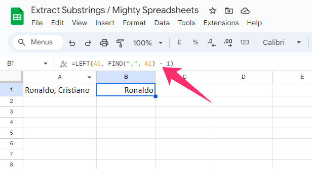
- Step 4: Enter the “=LEFT(A1, FIND(“,”, A1) – 1)” formula in the fx field.
- Step 5: Hit enter, and you’ll get “Ronaldo” as the output in the B1 cell.
Note: Like the “LEFT” function, this formula will also it from the beginning. But you’ll get an error if you use the same symbol or the text identifier more than once in the string.
Method 5: Get The Substring After Certain Text
Like before a certain text or symbol, Google Sheets also gives you the option to extract substrings after certain text or symbol. And you can do it easily by combining the “RIGHT,” “FIND,” and “LEN” functions.
Here, we will be using the “=RIGHT(<String identifier>,LEN(<String identifier>) – FIND(“<Text identifier>”,<String identifier>)-1)” formula.
The “String identifier” here is the cell or string from where you want to extract the substring. The “LEN” function enables Google Sheets to calculate the length of the string. And the “Text identifier” is the actual text or symbol before which you want to extract the substring.
We are using the “-1” option to eliminate the empty space before the text or symbol identifier.
Example: We will again work with the same “Ronaldo, Cristiano” example in the A1 cell. We want to get the output in the B1 cell. But instead of the surname, we will try to fetch the first name with this formula.
We will use the “Comma” sign as the text identifier and will also use -1 to eliminate the space after the comma sign. And the steps are as follows.
- Step 1: Click on the cell where you want to get your output (Here, it is B1).
- Step 2: Select the Formula (fx) field.

- Step 3: Enter the “=RIGHT(A1, LEN(A1) – FIND(“,”, A1) – 1)” formula (A1 is our string identifier, and the “,” sign is our text identifier).
- Step 4: Hit the Enter button, and you’ll get “Cristiano” as the output in the B1 cell.
You can also use the “SEARCH” function instead of the “FIND” function to extract the substring using the same formula as well. Besides, you can also use other functions to modify this formula to get a tailored output.
Note: You can now automatically assign numbering in rows which can be extremely helpful while working with a complex sheet with a large amount of data. So, don’t miss my detailed guide on automatically number rows in Google Sheets.
Using Regular Expressions For Advanced Substring Extraction
If you are looking for a tested way to extract an advanced level or complicated substring from a particular string, regular expressions can be a savior here. It helps you to structure complex formulas.
What Is Regular Expression?
Regular Expression (or RegEx/REGEX) is a group or pattern of characters consisting of letters, numbers, and symbols. There can be any meta-character in a regular expression. You can combine these meta-characters to assign it as a search string or to use it inside a formula.
The regular phone number that comes in “Country code-City code-Phone number” format (E.G., 91-033-24448080) can be interpreted as “\d{2}-\d{3}-\d{8}” in the regular expression.
Here it is assigned 2 for the two digits in country code, assigned 3 for the next three digits representing city code, and assigned 8, which is the total character limit of a phone number in this format.
You can find more details about Regular Expressions on the Google support page.
Some Common Examples Of Regular Expressions
Although there are many regular expressions available, you can use a handful of them to technically do almost anything on Google Sheets. And the most used regular expressions are as follows.
| Regular Expression | Commonly Called | Representation |
| ^ | Caret | The start or the beginning of any string |
| $ | Dollar Sign | The end of any string |
| . | Dot | Denoting a single character in the string |
| | | Pipe | Matches two alternative blocks in a string |
| ? | Question Mark | Zero or single occurrence in a string |
| + | Plus Sign | One or more occurrences in a string |
| <Space> | Empty Space | Include all the white spaces in a string |
| () | First Bracket | Includes a group of meta-characters |
| [] | Third Bracket | Holds a group of real characters or texts |
| […] | Continue Sign | Matches any character within a group of characters |
REGEXEXTRACT Function In Google Sheets
You can now also use the REGEXEXTRACT function in Google Sheets to extract a matching substring from a particular string. And here, you can use the regular expression meta-characters to write the formula.
The main formula we will be using here is “=REGEXEXTRACT(<String identifier>,“<Regular Expressions>”).”
The string identifier in this formula is the cell or range from where you want to extract the substring. And in the regular expression field, you can use any possible variation of available expressions.
Example: We have a phone number, “+91-033-24448080,” in the A1 cell and want to extract the last four digits as the output in the B1 cell.
So, we will use four dots (.…) as the first regular expression, as each dot represents a single digit/character in REGEX. And we will combine it with $, as we want to extract the substring from the end. The steps are as follows.
- Step 1: Launch Google Sheets and open your spreadsheet.
- Step 2: Click on the empty output cell (Here it is B1).
- Step 3: Click on the Formula (fx) field.
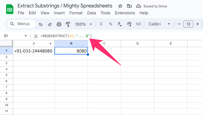
- Step 4: Enter the “=REGEXEXTRACT(A1,”….$”)” formula.
- Step 5: Hit the enter button, and you’ll get “8080” as the output in the B1 cell.
If you have an alphanumeric string or a string with both words and numbers, you can easily extract just the numbers by using the \d+ regular expression. You need to use the “=REGEXEXTRACT(<String identifier>,” \d+”)” formula to get the output.
Bonus: If you are collaborating with your team on Google Sheets, it is very important to keep a tab on the edit history. So, don’t miss my detailed guide on how to see edit history in Google Sheets.
Some Interesting Examples You May Like
There are many ways to extract substrings from a string in Google Sheets. And we have already shown six such ways that are extremely useful in different cases. But to make your life even easier, let’s check out some real-life examples.
Find A Substring Between Two Characters In Google Sheets
We have “Mighty Spreadsheet [+91-033-24448080]” in the A1 cell, which is a combination of the company name along with the phone number of the company within third brackets.
We will now extract just the phone number in the B1 cell as the output, as the phone number sits between two characters (bracket). The steps are as follows.
- Step 1: Click on the output cell (Here it is B1).
- Step 2: Click on the Formula (fx) field.
![=MID(A1,SEARCH([,A1)+1,SEARCH(],A1)-SEARCH([,A1)-1)](https://mightyspreadsheets.com/wp-content/uploads/2023/10/MIDA1SEARCHA11SEARCHA1-SEARCHA1-1.jpg)
- Step 3: Enter the “=MID(A1,SEARCH(“[“,A1)+1,SEARCH(“]”,A1)-SEARCH(“[“,A1)-1)” formula.
- Step 4: Hit the enter button, and you will get “+91-033-24448080” as the output in the B1 cell.
Here, we have combined the MID function with the SEARCH function to search particular characters first and then extract the substring between those characters.
Extract A Number From The String In Google Sheets
This time we have “Mighty Spreadsheet 24448080” in the A1 cell, which is a combination of a company name and the phone number. And we want to extract just the phone number in the B1 cell.
As we need the phone number as a value, we’ll combine VALUE and REGEX functions together. The steps to do it are as follows.
- Step 1: Click on the output cell (We are using B1 here).
- Step 2: Click on the formula (fx) field.
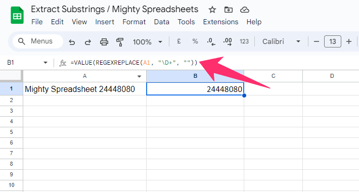
- Step 3: Enter the “=VALUE(REGEXREPLACE(A1, “\D+”, “”))” formula in the fx field.
- Step 4: Hit the enter button, and you’ll get “24448080” as the output in the B1 cell.
The regular expression \D+ can also be written as \d+. You can also use the [:digit:] regular expression as it will denote any number from 0 to 9 in any possible combination.
Note: It is now possible to directly collaborate with your teammates and colleagues right on the Google Sheets itself. Check out my latest guide on how to collaborate in Google Sheets to know more.
Get The First Character In Google Sheets
Let’s do something very interesting now! We have “All Day I Dream About Sports” in the A1 cell. Now, we want to extract the first letter of each word and then join them to get the output in the B1 cell.
So, we will use the LEFT function and the SPLIT together first in the formula to extract the first characters. And then, we will use the ARRAYFORMULA function to extract the first letters of multiple words. Finally, we will use the JOIN function to combine those.
You can also use the IFERROR function to avoid errors in case of a blank field. But to keep it simple, I’m using just four. And the steps are as follows.
- Step 1: Launch Google Sheets and click on the output cell (We are using B1 here).
- Step 2: Click on the formula (fx) field.
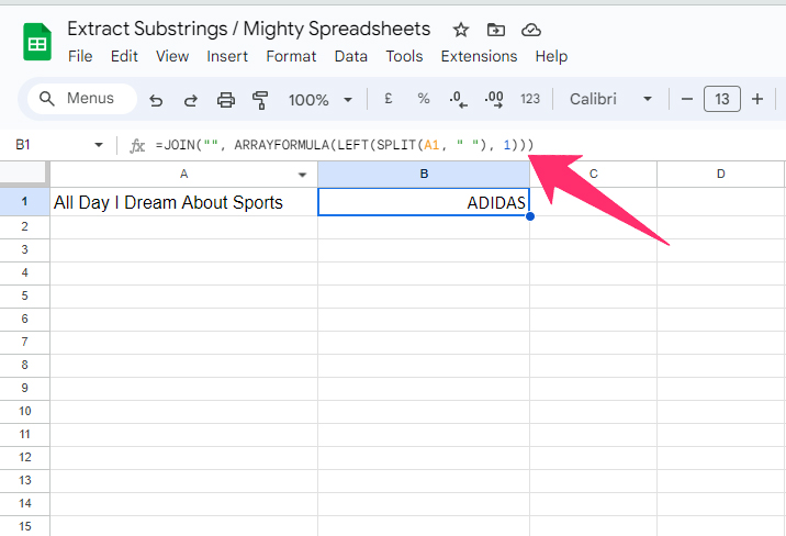
- Step 3: Enter the “=JOIN(“”, ARRAYFORMULA(LEFT(SPLIT(A1, ” “), 1)))” formula (Because our main string is on A1).
- Step 4: Hit enter, and you’ll get “ADIDAS” as the output in the B1 cell.
We can also use the “=ARRAYFORMULA(REGEXREPLACE(proper(A1),” [^A-Z]+”,””))” formula to get the same output. Instead of the exact string, we have used regular expressions here to make it more versatile.
Bonus: If you are working with a complex spreadsheet containing hundreds of data, you need to check for duplicates first to simplify it. I’ve already discussed all the tested methods in my comprehensive guide about removing duplicates in Google Sheets.
Key Takeaway
Unless you are trying to fetch something very complex, like an alphanumeric code or anything specific inside a bracket, you can easily extract substrings by using the LEFT, RIGHT, and MID functions in Google Sheets. Although they are not very versatile, they are easy to use and integrate.
But for complex extractions, you must use regular expressions to make your formula simple and also to accommodate more parameters in a single formula. And to first extract and then arrange some substrings in a particular form, it is better to use the ARRAYFORMULA along with the regular expressions.