How To Select Multiple Cells In Google Sheets?

At times, it becomes a necessity to select multiple cells, rows, and even columns to ensure a concise workflow. It is also necessary if you are working with complex data where you need to work with certain cells while leaving others intact. But do you know how to select multiple cells in Google Sheets?

You can simply click and then drag your mouse diagonally to select all the adjoining cells. Besides you can also use the “Shift + Click” or “Shift + Arrow keys” to do the same. Besides, you can replace “Shift” with “Ctrl” or “Cmd” to do the same for non-adjoining cells. To select matching cells of a particular value, you can use the “Find and Replace” option.

However, there are many other ways to select and highlight multiple adjacent and non-adjacent cells, rows, and columns in GS. So, without any further ado, let’s check out the easiest methods!

How To Select Multiple Cells In Google Sheets?

There are many ways to select certain cells in Google Sheets, depending on the requirement you have. But here, we have summed up the three easiest methods that anyone can try!

1. Click-And-Drag Method

If you don’t know how to select cells in Google Sheets, you should start with the traditional click-and-drag method. It is also the easiest way to select adjoining cells.

• Step 1: Launch Google Sheets and open your spreadsheet.
• Step 2: Click on the first cell of the cell range you want to select.

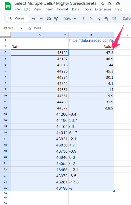
• Step 3: Click, hold, and then drag the mouse diagonally (upward or downward).
• Step 4: Release your mouse when you reach the last cell of your selected cell range.
• Step 5: You can now see your whole cell range is selected.

This is the way to select multiple adjoining cells in adjoining columns. If you want to select adjoining cells of a single column, hold and drag the mouse upward and downward to do the same.

This method works for both the with-value and non-value (empty cells). 

Bonus: You can now decorate your spreadsheet with amazing emojis and special characters, which will make it perfect for any presentation. Don’t miss my detailed guide on inserting emojis and symbols in Google Sheets.

2. Holding Down The “Ctrl” Key And Clicking On Cells

At times, you may need to select non-adjoining cells or rows in Google Sheets. But clicking and dragging won’t do the trick in that case. And you need to use a different method to do that.

• Step 1: Click to select the first cell of the cell range you want to select.
• Step 2: Press and hold the “Ctrl” button on your keyword.

• Step 3: Click on all the cells one by one without releasing the “Ctrl” key.
• Step 4: Once all cells are selected, release the control button.

This method will also work if you want to select multiple non-adjoining rows and columns. You need to first select a single row. Press and hold the “Ctrl” key and start clicking on all the rows or columns you want to select.

If you are using a Mac, you can do the same trick by pressing and holding the “Cmd” (Command) key.

3. Using The “Shift” Key To Select Multiple Cells At Once

If you want to select multiple adjoining cells, you can do it pretty fast with the “Shift” key rather than the “Ctrl” key, where you need to click on every cell. The steps are easy, though!

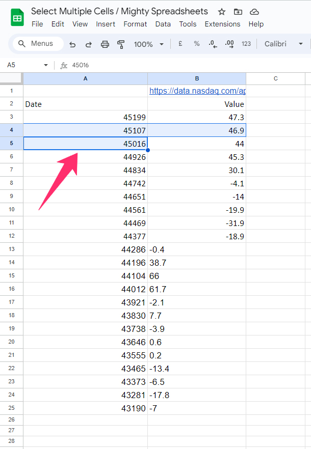
• Step 1: Click on the first cell of the cell range you want to select.
• Step 2: Now, press and hold the “Shift” key in your keyword.

• Step 3: Click on the last cell of the cell range while pressing down the “Shift” key.
• Step 4: This will select all the cells in the specific cell range.

Please note that this method will only work for a continuous selection of adjoining cells. However, once you have selected the entire cell range with the “Shift” key, you can then press and hold the “Ctrl” key and click on individual cells that you want to remove from your cell range.

Tips: Do you know that the “IF” function is highly versatile that can solve many of your conditional problems? Check out my latest guide on the “IF” formula in Google Sheets to know more.

3 Advanced Techniques For Selecting Multiple Cells In Google Sheets

You may need different kinds of selections in Google Sheets, especially while working with complex data. And besides the three simple methods we have already mentioned, there are three more advanced methods also available.

1. Use The “Select All” Feature

Selecting the entire spreadsheet becomes necessary at times, especially if you want to set a filter or go with conditional formatting. And there are two ways to do that.

• Step 1: Open the spreadsheet on Google Sheets.
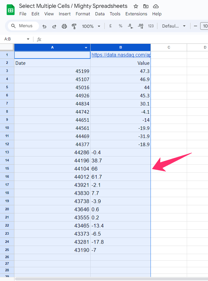
• Step 2: Navigate to the “Sheets Origin” cell located just below the “Name Box” and on the left side of the first (A) row.

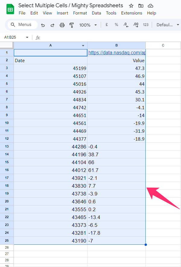
• Step 3: Click on it, and it will select all the cells in the spreadsheet at once.
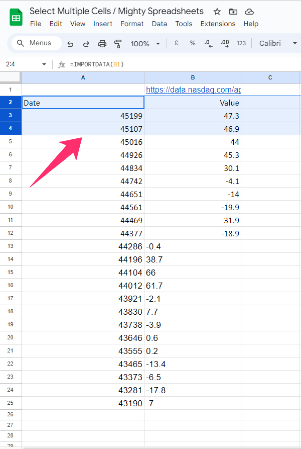
• Step 4: Alternatively, you can select just one cell in the spreadsheet.
• Step 4: Press “Ctrl + A” (for Windows) or “Cmd + A” (for Mac).
• Step 6: You can now see the entire spreadsheet is selected and marked in light blue.

Bonus: Do you know that you can now apply a specific formula to entire columns in Google Sheets? Don’t miss my newest guide on applying a formula to an entire column.

2. Using The “Find And Replace” Feature To Select Cells With Specific Values

If you want to select all the cells with specific values, there is a way to do it in Google Sheets. And that is by using the “Find And Replace” feature. The steps are as follows.

• Step 1: Launch Google Sheets on your computer and open your spreadsheet.
• Step 2: Click on the “Edit” button on the header menu and then on the “Find and Replace” option.

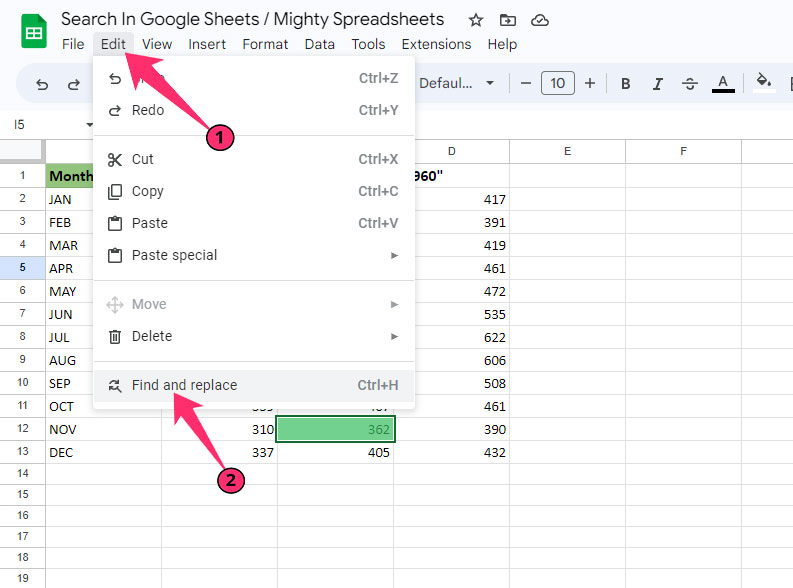
• Step 3: Alternatively, you can launch the “Find and Replace” feature by pressing the “Ctrl + H” (For Windows) or “Cmd + Shift + H” (For Mac) buttons.
• Step 4: Once you get a new popup window, type the value in the blank field beside the “Find” option.

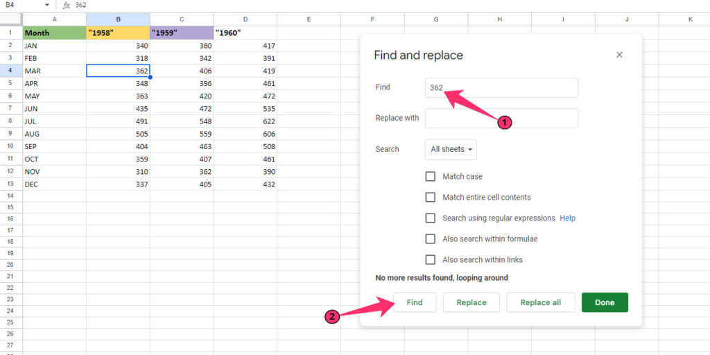
• Step 5: Click on the drop-down menu beside the “Search” header and select the “This Sheet” option (You can also select “All sheets” and “Specific range” depending on your needs.
• Step 6: Click on the “Find” button, and it will automatically select the first cell that matches the value.
• Step 7: You can proceed with selecting the next matching cells by clicking the “Find” button.

The “Find” option gives you five sets of filtering options. And you can choose among those filters according to your specific needs.

• Match case: It will make your search case-sensitive for every matching cell.
• Match entire cell contents: You’ll find the cells that have the exact match of the value.
• Search using regular expressions: You can search for a matching pattern using regular expressions.
• Also search within formulas: It will also search inside the formulas to find the matching values.
• Also search within links: With this one, you can search the matching value within a link.

This feature also gives you the scope to “Replace” a value with another “value” in every matching cell. For that, just press the “Replace” button instead of the “Find” button. Clicking on the “Replace all” button will replace all the matching cells at once.

3. Keyboard Shortcuts To Select Cells For More Efficiently

Google includes new shortcuts from time to time to make Google Sheets more user-friendly. And there are several shortcuts available to select particular cells. Some of the most useful among those are as follows.

• Ctrl + A: It will select the entire spreadsheet.
• Shift + Arrow: You need to first select a cell. Then just press and hold the “Shift” key and use your arrow keys (left, right, up, or down) to select adjoining cells.
• Ctrl + Shift + Arrow: By using this shortcut, you can select the complete usable area of your spreadsheet. It will only select up to that row and column that has some values.
• Ctrl + J: It will select the name box. Once selected, you can then enter the entire cell range (e.g., A1:D10), and it will select the specific range.

Please note that there is no shortcut available to select specific non-adjoining cells in Google Sheets. You can only do it by holding down the “Ctrl” or “Cmd” key and then clicking on the individual cell.

How To Select All Rows In Google Sheets?

We have already discussed how to select multiple boxes or cells on Google Sheets. Now, it’s time to uncover the ways to select multiple rows and columns. And depending on your need, there are three distinct methods available.

1. Select Multiple Rows In Google Sheets

You can now select all rows below or above a particular row in Google Sheets. You need to just use the “Shift” key to do it. And the steps are really easy!

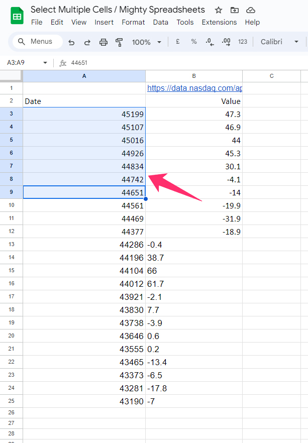
• Step 1: Click on the row name tab to select the first row of the range you want to select.
• Step 2: Press and hold the “Shift” key on your keyboard.

• Step 3: Use the down arrow key to select adjoining rows below the first row while holding the “Shift” key.
• Step 4: Alternatively, you can click on the adjoining rows while pressing the “Shift” key.
• Step 5: Both these methods will select multiple rows.

You can also select a row anywhere in the spreadsheet and then use both the “Up” and “Down” arrow keys to select multiple adjoining rows.

Bonus: It is now possible to directly collaborate with your teammates and colleagues on Google Sheets. Have a look at my latest guide on collaborating in Google Sheets to know more!

2. Select Multiple Columns In Google Sheets

Like rows, you may also need to select multiple columns in Google Sheets at once for a faster work process. And doing this is as easy as the first method!

• Step 1: Launch Google Sheets and click on the header of any column to select it.
• Step 2: Now, press and hold the “Shift” button on your keyboard.

• Step 3: Use the left or right arrow keys to select adjoining columns.
• Step 4: You can also keep on pressing the “Shift” key and then click on the adjoining column headers to select those.

Alternatively, you can just select one of the column headers of the range you want to select. And then, click and drag the mouse sidewise (left or right) to select multiple adjoining columns.

3. Selecting Multiple Non-Adjacent Rows Or Columns

You must have already understood by this point that selecting adjoining rows and columns is easy in Google Sheets. But at times, you may need to select multiple non-adjoining rows or columns. And there is an easy workaround!

• Step 1: Launch Google Sheets and open your spreadsheet.
• Step 2: From the cell range that you want to select, click on any row header to select it.
• Step 3: Press and hold the “Ctrl” (For Windows) or “Cmd” (For Mac) button on your keyboard.
• Step 4: Now, click on all the row headers you want to select individually.
• Step 5: You can also do the same thing with columns. Start with selecting a column header.
• Step 6: Keep on pressing the “Ctrl” or “Cmd” keys.
• Step 7: Click on the column headers that you want to select one after another.

Tips: You can now easily group specific rows and even columns in Google Sheets for an easy workflow. Check out my complete tutorial of grouping and collapsing rows and columns in Google Sheets to know in detail.

How To Highlight Multiple Cells, Rows, And Columns In Google Sheets?

Not only select, but you may also need to highlight certain cells, rows, or columns in your spreadsheet. And if you don’t know how to highlight two different columns or rows in Google Sheets, there are, again, three unique methods available to do that.

How To Highlight Two Adjacent Columns In Google Sheets?

You can now easily highlight two adjacent columns in Google Sheets in any color for an easy workflow. And the steps are also easy as well!

• Step 1: Open your spreadsheet in Google Sheets.
• Step 2: Click the column header of the first column of the range you want to select.
• Step 3: Press and hold the “Shift” key on your keyboard.
• Step 4: Now, click on the adjacent column header that you also want to select.
• Step 5: Release the shift key, and two adjacent columns will be selected.

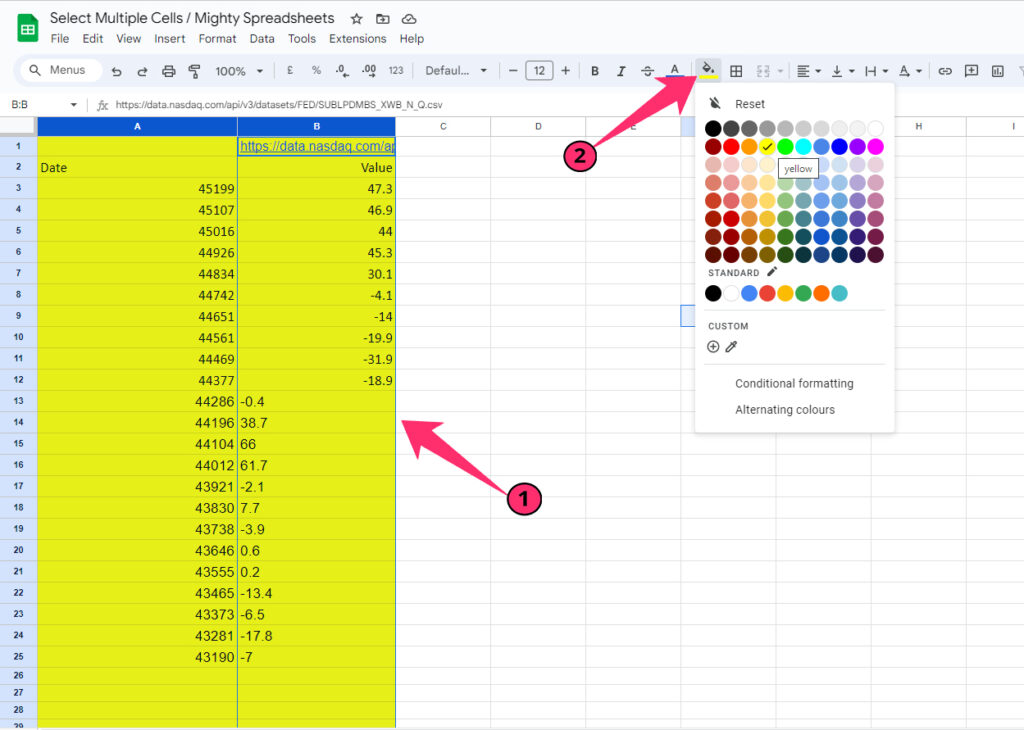
• Step 6: Click on the “Fill color” option from the header menu.
• Step 7: Select any color you want from the pallet, and two selected adjoining columns will be highlighted.

You can also use the left or right arrow keys to select adjacent columns instead of clicking with the mouse while holding down the “Shift” key. Besides, this operation can also be done with “Ctrl” or “Cmd” in the same way.

How To Highlight Two Separate Columns In Google Sheets?

There are many ways to highlight two different (even non-adjoining) columns in Google Sheets. First, you can do it by holding down the “Ctrl” or “Cmd” key and then clicking on both the column header to select those. You can then highlight those columns with any color.

But, if you want to highlight certain matching rows, you can use the conditional formatting option to do it. The steps are also not very complicated.

• Step 1: Open your spreadsheet and click on the “Format” option on the header menu.

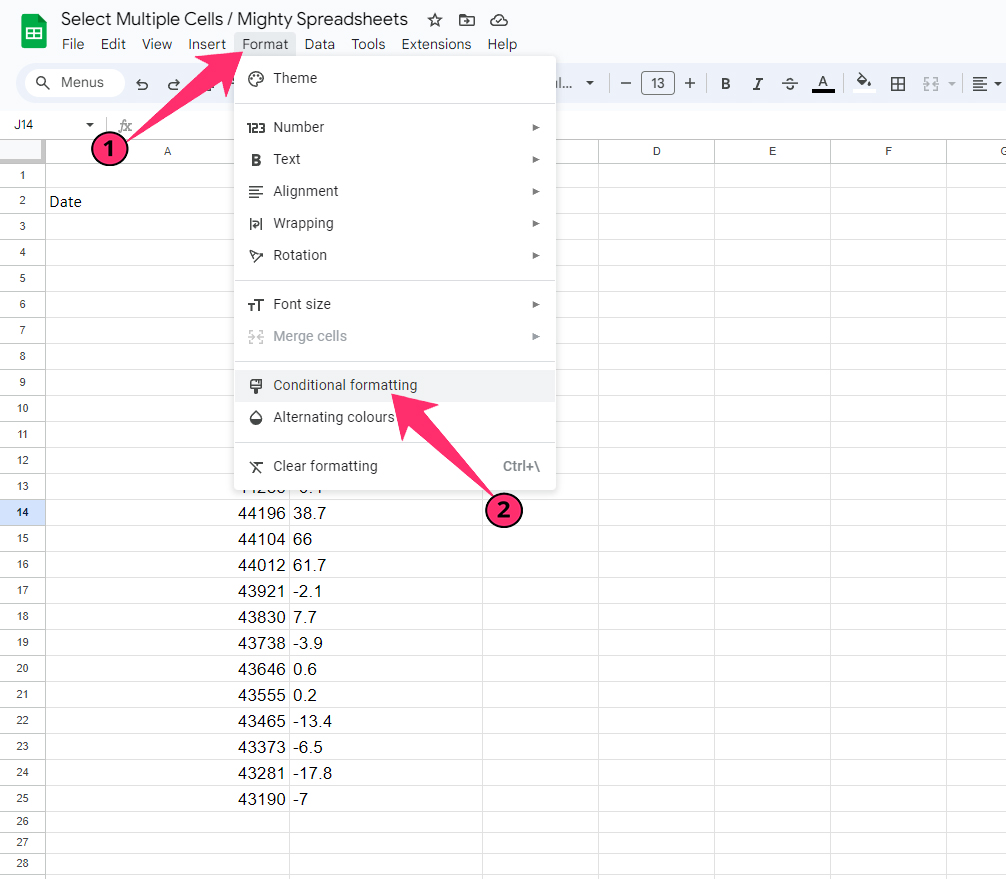
• Step 2: Click on the “Conditional Formatting” option.
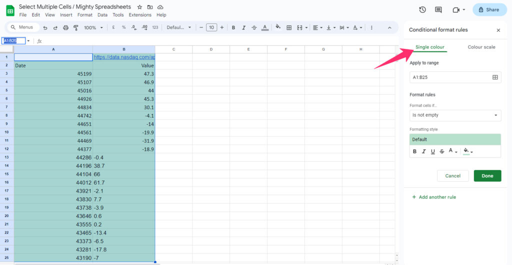
• Step 3: This will bring a sidebar named “Conditional Format Rules” on the right side of your spreadsheet.
• Step 4: Select “Single color” from the header tag (it is the default).
• Step 5: Click on the “Apply to range” option (grid symbol), and a small popup window will appear.

• Step 6: Type your cell range in “<first cell>:<last cell>” format and click on the “OK” button. (You can also add multiple ranges).
• Step 7: Now, select your filtering parameter from the drop-down menu under the “Format cells if…” header (you can select only one filtering option at a time).
• Step 8: Click on the “Fill color” option under the “Formatting styles” header.
• Step 9: Select any color of your choice from the pallet (you can even use custom colors).
• Step 10: Click on the “Done” button, and all the matching columns in the selected range will be highlighted.

You can even search for a specific formula in a spreadsheet using this same method. Just use the “Custom formula is” option and then put the formula in the designated field. This will do the trick!

How To Highlight Multiple Rows In Google Sheets?

Yes, it is also easy to select and highlight multiple adjoining or non-adjoining rows in Google Sheets. And it is as easy as working the columns which we have already mentioned above.

• Step 1: Launch your spreadsheet in Google Sheets.
• Step 2: Click on any row header from the range you want to select.
• Step 3: Now, press and hold the “Shift” key (for adjoining rows) or the “Ctrl/Cmd” key (for non-adjoining rows).
• Step 4: Click on all the row headers one by one while pressing the button in your keyword.
• Step 5: This will select all the rows that you want to highlight.

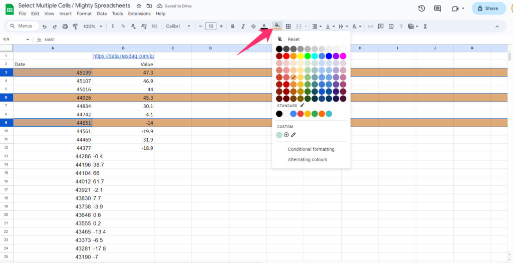
• Step 6: Click on the “Fill color” option from the header menu.
• Step 7: Choose any color from the pallet, and this will highlight all the selected rows.

If you want to select and highlight adjacent rows, you can also use the up and down arrow keys instead of clicking while holding down the “Shift” key. This will also select adjoining rows.

How To Select Multiple Cells In Google Sheets Mobile App? (iPhone, iPad, Android)

It is easy to use shortcuts and mouse cursors for better productivity in Google Sheets on desktops and laptops. But it is not the same if you talk about the mobile app.

Although it is highly versatile, you will miss certain features. But yes, there is a way to select multiple cells easily, even on the Google Sheets mobile app.

• Step 1: Launch the Google Sheets app on your smartphone and open your spreadsheet.
• Step 2: Click on the “Name box” right beside the function (fx) bar and under the header menu.
• Step 3: Enter your desired cell range in the “<first cell>:<last cell>” format.
• Step 4: This will select all the cells in your range.

Tip: What will you do if you want to know which revision is done by whom in your teammate in Google Sheets? There is an easy way to do that. Check out my latest guide on how to see the complete edit history in Google Sheets to know the details.

Final Note

If you don’t want to select certain cells, rows, or columns that match a certain value or parameter, rather, you want to select just adjoining cells, it is better to use easy methods.

Using the “Shift” and “Ctrl” keys with the arrows or mouse click will serve most of your purpose. Besides, it is also better to use the “Name box” to select a particular cell range at a much faster speed.

But if you want to select cells with matching values, conditional formatting is the best option. It also works well in the Google Sheets app besides the web version.

Some Questions You May Have

How To Select All Cells Containing A Value?

If you want to select cells with any value, you can easily do it by clicking on the blank cell right on the left beside the column “A” header (beneath the name box). But if you want to select just matching cells of a specific value, you can do it with either “Find and Replace” or “Conditional formatting.”

How To Select A Range Of Cells In Google Sheets?

You can easily select a particular range of cells by using the name box in Google Sheets. It is located on the left side of the “function” field. Just enter the cell range in the name box in the “<first cell of the range>:<last cell of the range>” format.