Make Google Sheets Random Number Generator (In Less Than 1 Minute)

In this article, you’re going to discover how to create a random number generator in Google Sheets – a surprisingly simple yet handy feature that can be accomplished in no time.

Remember, though, each of these functions is designed for a specific use case and they are quite volatile in nature, meaning that they will recalculate with every change in the worksheet.

Let’s now dive into a step-by-step guide that will help you master these formulas and start generating random numbers in Google Sheets effortlessly.

Make A Random Number Generator Using The “RAND” Function

Transforming your Google Sheets into a random number generator isn’t a complicated task. And it allows you to produce random integers and decimals without any noticeable patterns. This article will provide a straightforward guide to generating these random numbers in Google Sheets.

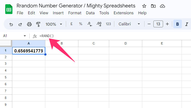
Firstly, open Google Sheets and identify the cell where you want to produce a random number. Navigate to the “Formula” field (fx) and input the =RAND() function. Once you hit the “Enter” button, a random decimal number between 0 and 1 will appear.

Typically, this method generates a number with ten decimal digits. However, you can adjust the decimal count using the “Round” function. For instance, the formula “=ROUND(RAND(),<desired decimal places>)” will round off the number to your specified decimal places.

Here’s how to produce a random number up to the third decimal place:

1. Select the cell and input the =RAND() formula.
2. Edit the formula to =ROUND(RAND(),3) limit the output to three decimal places.

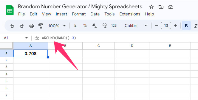
Just replace ‘3’ with your preferred decimal digit in the formula – for the second decimal place, use =ROUND(RAND(),2), and for the fifth, use =ROUND(RAND(),5)

If you need to generate multiple random numbers, there’s no need to repeat this process. Input the formula in the first cell and drag the fill handle (the small square at the bottom-right corner of the cell) to the desired end cell.

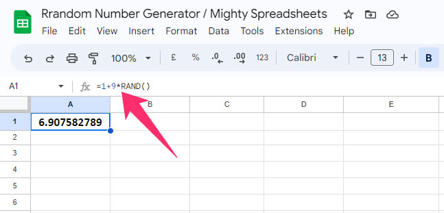
Note that the “RAND” function produces values in the fractional part only, without any whole number. However, you can adjust this function to generate random numbers between 1 and 10, including whole numbers and fractions (e.g., 2.52369 or 7.36598). You can also further modify it to round off these numbers to a specific number of digits.

Follow these steps to do this:

1. Select a cell and navigate to the “fx” field.
2. Input the formula =1+9*RAND() and press enter.
3. This action will produce a random number between 1 and 10, including whole numbers and fractional digits.
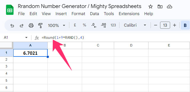
4. To round off this number to the fourth decimal place, input the formula =ROUND(1+9*RAND(),4) and press enter.

In summary, the formula =ROUND(1+9*RAND(),<desired decimal places>) combines three functions.

First, =RAND() produces a random number, which is then modified to =1+9*RAND() This operation multiplies the random fractional number by 9 and adds 1 to the result.

Lastly, =ROUND(1+9*RAND(),4) rounds off this number to your chosen decimal place.

A word of caution: using different formulas in different cells might result in duplicate random numbers. However, you can quickly remove these duplicates, as explained in my latest guide on managing duplicates in Google Sheets.

Change Recalculation Settings for Random Number

While Google Sheets provides a convenient platform for generating random numbers with the methods I’ve outlined above, the “RAND” function is quite volatile.

In other words, any alterations made to the sheet or simply reloading the page will trigger a new set of values.

This can lead to slower performance, particularly when handling large data sets. Luckily, you can modify the “Recalculation” settings to manage this situation.

Here’s a step-by-step guide to adjust your recalculation settings:

Step 1: Launch the sheet where you have inserted the “RAND” formula.

Step 2: Click on the “File” option in the header menu.

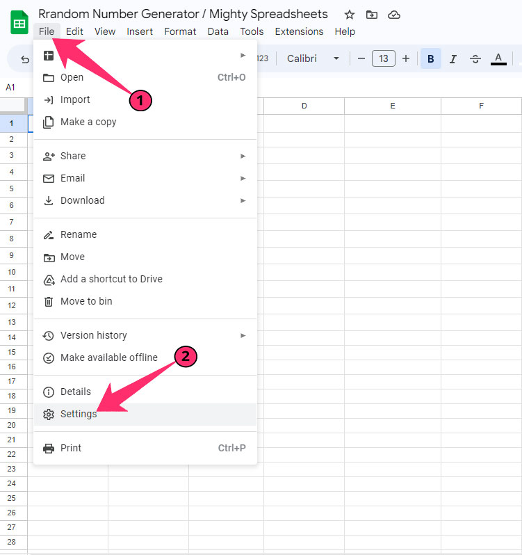
Step 3: From the dropdown list, select “Settings,” and a popup menu will appear.

Step 4: Navigate to the “Calculation” option in the header menu.

Step 5: Click on the dropdown menu under the “Recalculation” option.

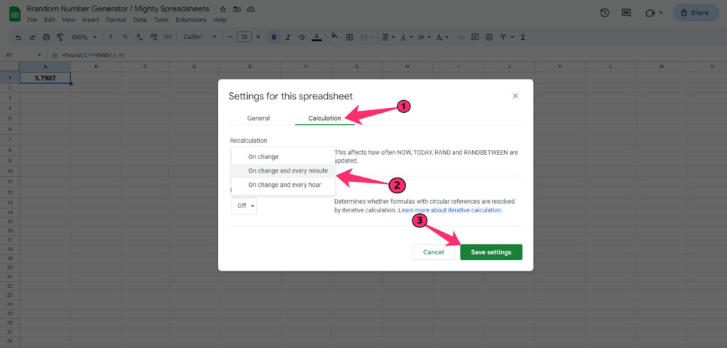
Step 6: Select among “On change,” “On change and every minute,” and “On Change and every hour” options.

Step 7: Click on the “Save settings” button at the bottom-right corner. 

Note: Bear in mind, these adjustments to the recalculation settings are not limited to “RAND” and “RANDBETWEEN”; they also apply to time functions like “TODAY” and “NOW.” Check out my most recent guide on time operations in Google Sheets for more in-depth information.

How To Generate A Random Number That Fits Between Two Numbers?

You must have already understood how to make a random generator in Google Sheets using the “RAND” formula.

However, there might be cases when you need to generate numbers within a specific range, say between 5 and 6. This is where the RANDBETWEEN formula comes into play!

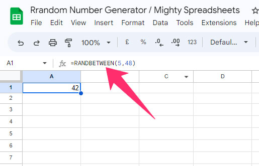
Here’s the syntax: =RANDBETWEEN(<lower_limit>,<upper_limit>

The lower limit sets a floor for the generated numbers, meaning that the random numbers produced will be equal to or greater than this limit.

Conversely, the upper limit sets a ceiling for the random numbers. Thus, any generated number will be equal to or less than this limit.

Remember, the upper limit should always exceed the lower limit.

It’s important to note that both the upper and lower limits need to be integer values, as the formula doesn’t accommodate fractional numbers.

Use Custom Formula (To Generate Random Decimal Numbers)

You can easily tweak the “RAND” formula and make some changes to generate decimal numbers with positive integer values. And the steps are pretty easy!

• Step 1: Launch Google Sheets and click on the cell where you want to generate random decimal numbers within two ranges.
• Step 2: Click on the “fx” field to enter the formula.
• Step 3: Put the “=RAND()*(<upper limit – lower limit>)+<lower limit>” formula.

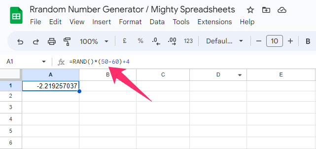
• Step 4: Hit the “Enter” button, and a random decimal number will appear on that cell.

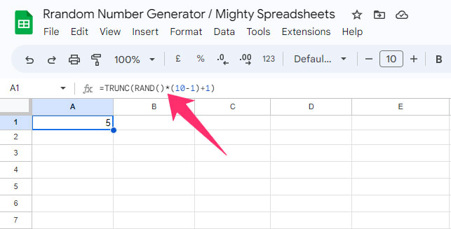
Explanation: Let’s say I want to generate random decimal numbers between 1 and 10. The formula will be “=RAND()*(10-1)+1)” here, where the upper limit is 10, and the lower limit is 1.

The core “=RAND()” function will first generate a decimal value without a whole number before the decimal. The formula will then multiply the value with the difference between the upper and lower limit. 1 will be added in the second output to make sure it contains a whole number before the decimal sign.

You can also remove the fractional part from the random number by tweaking the formula even further. We will use the “TRUNC” function for that. Steps are again easy!

• Step 1: Select a cell and click on the “fx” field.
• Step 2: Enter the “=TRUNC(RAND()*(<upper limit–lower limit>)+<lower limit>)” formula.

• Step 3: Hit the “Enter” button, and it will generate a random integer between the limits.

Explanation: If you want to generate a random integer between 1 and 10, the formula will be “=TRUNC(RAND()*(10-1)+1).” But like the RAND function, you need to enter both the limits in whole numbers. Besides, the upper limit should be bigger than the lower one.

Note: If you want to work under a certain range of values, you can now even do that in Google Sheets. Follow my latest tutorial on how to lock cell ranges in Google Sheets to know more about it!

Use “RANDBETWEEN” (To Generate A Whole Random Number)

Google Sheets offers another function called “RANDBETWEEN,” with which you can generate whole numbers pretty easily. And you can also set the ranges between which you want to generate the random whole number. Here are the steps.

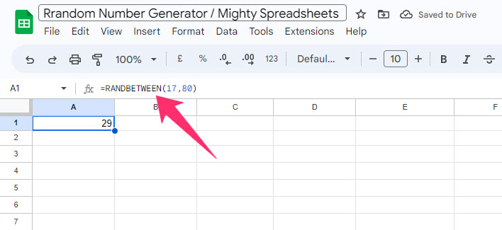
• Step 1: Open Google Sheets and click on an empty cell.
• Step 2: Click on the “fx” field and enter the “=RANDBETWEEN(<lower limit>,<upper limit>)” formula.

• Step 3: Press the “Enter” button, and a whole number will appear in the designated field.

Both the upper and lower limit should be whole numbers to make this formula work. However, if you are working with a data set and want to set the values of certain cells as your lower and upper limit, you can even do that.

• Step 1: Click on the empty cell and then on the “fx” field.
• Step 2: Enter the “=RANDBETWEEN(<cell name of the lower limit>,<cell name of the upper limit>)” formula.

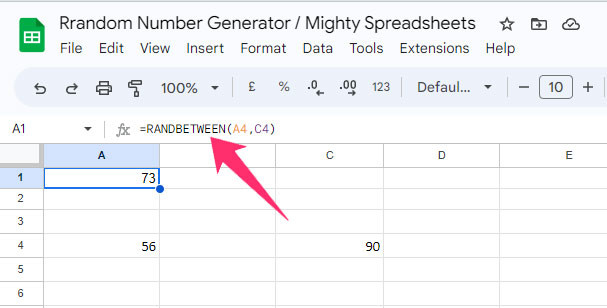
• Step 3: Hit the “Enter” button to generate a random whole number within the specified limit.

Explanation: Let’s say I want to use the value of the “A4” cell as the lower limit and the value of the “C4” cell as the upper limit. Then the formula will be “=RANDBETWEEN(A4,C4).” But you need to make sure that the C4 cell has a greater number than the A4 cell.

Differences Between RAND And RANDBETWEEN Functions

The “RAND” function is more versatile than the “RANDBETWEEN” function. And you can do many things by using “RAND” as your core formula. However, there are several differences.

RAND	RANDBETWEEN
It always returns decimal values	Only returns integer values
More likely to produce unique decimal numbers in a smaller range	Less likely to produce unique integers in a smaller range
It will not ask for any upper or lower limit	Always asks for the upper and lower limit
Generate decimals between 0 and 1	Generates integers within the specified range
Works well with other formulas	It can cause lag while using it with other formulas

You can easily replace the “RANDBETWEEN” function with “RAND” simply by tweaking the core formula. But it will be really hard to do the opposite.

RANDBETWEEN Function’s Limitations

The “RANDBETWEEN” function, while versatile and dynamic, does come with certain restrictions. Some of these limitations include:

1. It has the capability to generate random integers, but it often struggles to produce a unique set of integers without repetition.
2. This function performs best when the set limits have a wide range (e.g., between 1 and 10,000). However, when the range is relatively narrow (e.g., between 1 and 10), it begins to repeat integers.
3. As it only produces integer values, the “RANDBETWEEN” function is less versatile compared to the “RAND” function, which generates decimal numbers.
4. It may not function optimally with more complex formulas due to its inability to consistently generate unique numbers.
5. Large data sets can significantly slow down the performance of your Google Sheet when using the “RANDBETWEEN” function.
6. If you incorporate “RANDBETWEEN” into numerous formulas within a single sheet, this can also result in slower processing speeds.

However, it’s worth noting that both the “RAND” and “RANDBETWEEN” functions can be used effectively to generate unique random numbers.

Note: You can quickly generate unique random numbers with both RAND and RANDBETWEEN functions and then can filter the data. Check out my latest guide on filtering data in Google Sheets to learn more.

How To Create Random Arrays Using The “RANDARRAY” Function?

Using the “RAND” function, you’ve learned how to generate random numbers in Google Sheets without repetition.

While the “RAND” function doesn’t require arguments such as lower and upper limits, you can introduce these parameters by incorporating the “ARRAY” function. Here’s how:

1. Start by opening Google Sheets and clicking on an empty cell.
2. Click on the “Function” (fx) field.
3. In the provided space, type the formula =RANDARRAY(<Rows>,<Columns>).
4. Hit the enter key, and random numbers will immediately populate the specified cell range.

Let’s illustrate this with an example. Suppose you need random numbers across 10 rows and 3 columns. All you need to do is select the first cell and input the formula =RANDARRAY(10,3). Once you’ve entered the formula and pressed enter, random numbers will automatically fill the specified 3 columns across all 10 rows.

Some Questions You May Have

How to keep random numbers from changing in Google Sheets?

If you place a formula, such as RAND, RANDBETWEEN, or RANDARRAY, in cells, it will automatically change if you reload or make changes in the Google Sheets. You can stop that change by copying the values from those cells and then pasting those to blank cells. 

You can either use the “Ctrl + C” option or can also right-click on the cell and then select Paste Options>Values.

How to generate random numbers from a list?

Imagine having a list of 10 data points in cells A1 through A10 in Google Sheets, and you want to select a value at random from this list. This is achievable in just a few simple steps:

1. Click on any empty cell.
2. Type in the formula “=INDEX(A1:A10,RANDBETWEEN(1,10))”.
3. Press the enter key.

This formula will randomly select a value from the cells in your reference list (A1:A10). What happens here is that the “RANDBETWEEN(1,10)” function randomly generates a number between 1 and 10.

This number is then used as an index to select a cell from the range A1:A10.

The “INDEX” function then returns the content of the chosen cell. So each time you execute this formula, a different value from your list might be displayed.

Final Note

While the “RAND”, “RANDBETWEEN”, and “RANDARRAY” functions are extremely flexible, they are also highly volatile.

This means they recalculate and change their results every time there’s a change in the sheet or each time the sheet is reloaded.

Among these, “RAND” provides more customization options and is particularly well-suited for working with large data sets.

To preserve a specific output from these functions, it’s advisable to copy the value and paste it into an empty cell immediately after execution.

This way, you can ensure the number won’t change with each reload or restart of your Google Sheets.

This can be done simply by using ‘Paste as Values’ (right-click the cell, select ‘Paste special’, and then ‘Paste values only’).

This step is crucial if you need to retain a record of the random number generated for future reference.